Drawing Thick Lines
The Bresenham algorithm is a very nice one for drawing 1-pixel lines. It uses only addition and comparison and so runs very fast. However, it can't handle thicker lines. Alan Murphy has made a modification to Bresenham's algorithm for this purpose. The linked site includes part of a paper explaining the algorithm. The paper, his example code and his website are very terse. There is some explanation but you would understand them only if you were already very familiar with the subject. In this article, I'll try to re-discover his algorithm and make a complete implementation.Basic Bresenham Line
Let's assume that we have a line in the first octant (dx>dy>0). We will step thru the x coordinates. While stepping from left to right, we observe that the next pixel will be one of the following:- the pixel immediately to the right
- the pixel which is one pixel up and one pixel right
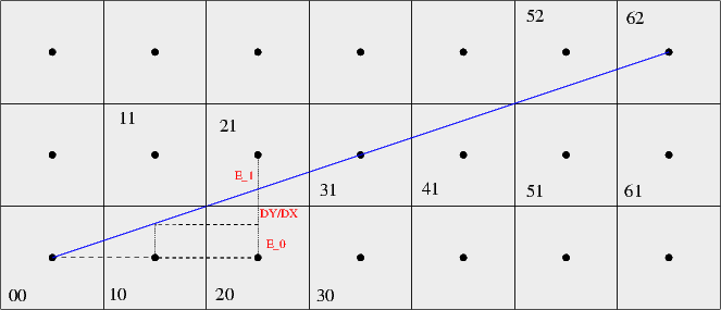
Let's assume we're moving from 00 to 10. When we increase the X coordinate, the error will increase by DY/DX. If the error becomes greater than 0.5, then the pixel above (11) should be selected. 0.5 is the distance between the center of a pixel and its top border. So, our step is:
  if (error+dy/dx > 0.5)
    y = y+1
  endif
If we make a right move, the error update is trivial:
error= error + dy/dxOtherwise, the error is calculated from the center of the pixel above. We observe that
E1+DY/DX+E0= 1
E1= 1 - E0 - DY/DX
However, the sign of the real error is negative, so we take that instead.
E1'= -1 + E0 + DY/DXWhich means that:
error = error + dy/dx - 1In order to get rid of dy/dx terms, we can easily multiply all values with 2dx. The condition and the updates become:
  if error + 2dy > dx
  error = error + 2dy
  error = error + 2dy - 2dx
Summing up, the algorithm becomes:
  error= 0
  y= y0
  for x = x0 .. x1
    pixel(x,y)
    if error + 2dy > dx
      y= y+ 1
      error = error - 2dx
    end
    error= error + 2dy
  end
So, let's put this in the Murphy format for later use:
thin_octant1(x0,y0,dx,dy):
  error= 0
  y= y0
  x= x0
  threshold = dx - 2dy
  E_diag= -2dx
  E_square= 2dy
  length = dx
  for p= 1 .. length
    pixel(x,y)
    if error > threshold
      y= y + 1
      error = error + E_diag
    end
    error = error + E_square
    x= x + 1
  end
A Simple Perpendicular
With the information above, let's see how we could draw a perpendicular to the blue line from (x0,y0). Let's consider the perpendicular going towards top left. Obviously, we will step on increasing y coordinates and decrease the x coordinate when necessary.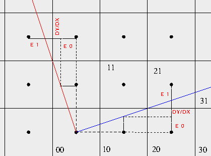
The error is again initially zero. The test for diagonal/square move is:
if error - dy/dx < -0.5The error update for square move is:
error= error - dy/dxand for the diagonal move:
  E1 + dy/dx - E0 = 1

here, we subtracted E0 because its sign is negative..

  E1 = 1 - dy/dx + E0

  error = error + 1 - dy/dx
Summing up,
  if error - dy/dx < -0.5
  error= error - dy/dx
  error = error + 1 - dy/dx
Something strange happens if we multiply all values with -2dx (instead of 2dx in the thin line algorithm).
  if error + 2dy > dx
  error= error + 2dy
  error= error - 2dx + 2dy
These are exactly the same things as the previous set of equations. So, our algorithm for the left-perpendicular is almost the same, only the coordinate updates are different.
thin_octant1(x0,y0,dx,dy):             pleft_octant1(x0,y0,dx,dy):
  error= 0                               error= 0
  y= y0                                  y= y0
  x= x0                                  x= x0
  threshold = dx - 2dy                   threshold = dx - 2dy
  E_diag= -2dx                           E_diag= -2dx
  E_square= 2dy                          E_square= 2dy
  length = dx                            length = ..desired-width..
  for p= 1 .. length                     for p= 1 .. length
    pixel(x,y)                              pixel(x,y)
    if error > threshold                    if error > threshold
      y= y + 1                                x= x - 1
      error = error + E_diag                  error = error + E_diag
    end                                     end
    error = error + E_square                error = error + E_square
    x= x + 1                                y= y + 1
  end                                    end
A Naive Thick Line
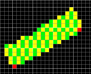
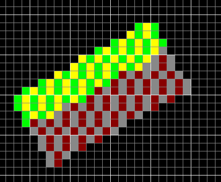
By using the above perpendicular function, we could maybe draw half of a thick line. Instead of calling pixel() in thin_octant1, we could call pleft_octant1 and draw a whole segment to the left instead of a single pixel. Let's do that and see what happens.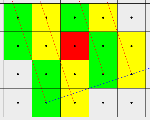
Here, the green and yellow squares represent pixels painted on alternate runs of the perpendicular loop. As you can see, no line passes thru the red square. This will happen every time the thick_octant1 increases y and thus makes a diagonal move. There are more red squares to the left and top, we could see those if the image was big enough.
Why does this happen? It's because the perpendicular lines start from the initial state (error=0) and don't follow each other. For example, consider the first green and first yellow sequence. They have the same phase at each y coordinate: they are essentially the same sequence since their initial y value is also identical. Whenever one makes a diagonal move, the other does it too. This way, there is no gap left between them.
The same thing doesn't happen with the first yellow and second green sequence. The yellow sequence does a diagonal move at y=1 but the green sequence does a square move since it's the very first move for that sequence. If I could somehow execute the same sequence at the same y coordinate, the problem would be solved.
The solution to this is to start all perpendicular lines not at (x,y) but at (x,y0) and draw only the part that falls to the left side of the blue line. I'm not going to draw it here. Just imagine that you layout copies of the first green line along the x axis. Obviously we wouldn't miss any squares. However, this isn't efficient or elegant. I should figure out how to calculate the perpedicular's error at (x,y) without going from (x,y0) to (x,y).
A Second Try
If you look at the definition of pleft_octant1 and thin_octant1, you will see that the blue line and the red line are actually identical. They are just rotated versions of each other. For the same 'p' value, the error is the same in both functions.We could calculate the 'phase' or 'accumulated error' of the perpendicular within the thick_octant1 function using the E_diag, E_square and threshold values. However, we update this error variable only when we make a diagonal move in the thick_octant1 function. When we make a square move, the y coordinate doesn't change and the next perpendicular should start with the same error we have now. When we make a diagonal move, y coordinate has changed and a new error should be calculated to decide whether we will go with the current x coordinate or one less in the perpendicular. So, our thick_octant1 should look like this:
thick_octant1(x0,y0,dx,dy):
  p_error= 0   # the perpendicular error or 'phase'
  error= 0
  y= y0
  x= x0
  threshold = dx - 2dy
  E_diag= -2dx
  E_square= 2dy
  length = dx
  for p= 1 .. length
    pleft_octant1(x,y, dx, dy, p_error)
    if error > threshold
      y= y + 1
      error = error + E_diag
      if p_error > threshold
        p_error= p_error + E_diag
      end
      p_error= p_error + E_square
    end
    error = error + E_square
    x= x + 1
  end
The new pleft_octant1 is almost the same as the old one. It just doesn't
initialize error to 0, it gets the initial value for it from the thick_octant1
function.
pleft_octant1(x0,y0,dx,dy,error):
  y= y0
  x= x0
  threshold = dx - 2dy
  E_diag= -2dx
  E_square= 2dy
  length = ..desired-width..
  for p= 1 .. length
     pixel(x,y)
     if error > threshold
       x= x - 1
       error = error + E_diag
     end
     error = error + E_square
     y= y + 1
  end
That's pretty much it, but one more issue remains. Before I go into that,
let's look at how this thing runs.
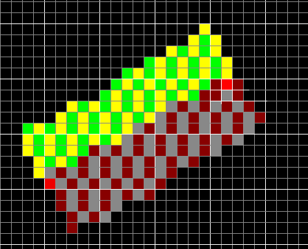
We managed to make all perpendiculars 'in-phase', i.e. all perpendiculars do the same thing (diagonal or square move) at the same y. However, some perpendiculars seem to be missing completely. This situation is what Mr. Murphy calls a 'double square move'.
In our particular example, the very first move is a diagonal one. We draw the first perpendicular (yellow) normally. Then we move on to the next start point using a diagonal move. Since our first move for the first perpendicular was also a diagonal move, we failed to cover the square right above the red square. In order to overcome this, we add another call to pleft_octant1 in the thick_octant1 function. Just where we detect this situation:
thick_octant1(x0,y0,dx,dy):
  p_error= 0   # the perpendicular error or 'phase'
  error= 0
  y= y0
  x= x0
  threshold = dx - 2dy
  E_diag= -2dx
  E_square= 2dy
  length = dx
  for p= 1 .. length
    pleft_octant1(x,y, dx, dy, p_error)
    if error > threshold
      y= y + 1
      error = error + E_diag
      if p_error > threshold
        pleft_octant1(x,y, dx, dy, p_error+E_diag+E_square)
        p_error= p_error + E_diag
      end
      p_error= p_error + E_square
    end
    error = error + E_square
    x= x + 1
  end
Here, we used the phase of the next perpendicular for the extra
perpendicular. This is because the extra perpendicular starts at the same
y coordinate as the next perpendicular. The remote end of the perpendicular
lines is jaggy, resulting in varying width. This is because we use number
of pixels travelled as our width measure, which is obviously incorrect due
to diagonal moves. Murphy has a solution for this too, namely using the
error variable as the measure. I will do this later. Below is the
current rendering:
Reverse Perpendicular
Now we have the left side of the thick line. We need to draw the right side also. For this, we need to travel the perpendicular in reverse direction. The following should be sufficient:- The error values will be subtracted instead of added to the current error.
- The error will be compared against -0.5 for diagonal decision.
- x and y coordinates will be updated in the reverse direction.
pleft_octant1(x0,y0,dx,dy,error):      pright_octant1(x0,y0,dx,dy,error):
  y= y0                                  y= y0
  x= x0                                  x= x0
  threshold = dx - 2dy                   threshold = dx - 2dy
  E_diag= -2dx                           E_diag= -2dx
  E_square= 2dy                          E_square= 2dy
  length = ..desired-width..             length = ..desired-width..
  for p= 1 .. length                     for p= 1 .. length
     pixel(x,y)                            pixel(x,y)
     if error > threshold                  if error < -threshold
       x= x - 1                              x= x + 1
       error = error + E_diag                error = error - E_diag
     end                                   end
     error = error + E_square              error = error - E_square
     y= y + 1                              y= y - 1
  end                                    end
If I do the multiplication trick using the value -1, I end up with the
following definition for pright_octant1:
pright_octant1(x0,y0,dx,dy,error):
  y= y0
  x= x0
  threshold = dx - 2dy
  E_diag= -2dx
  E_square= 2dy
  length = ..desired-width..
  error= -error
  for p= 1 .. length
    pixel(x,y)
    if error > threshold
      x= x + 1
      error = error + E_diag
    end
    error = error + E_square
    y= y - 1
  end
This is almost the same thing as pleft_octant1 except for the directions
of the coordinate updates. The underlined statement comes from the
multiplication by -1. I feel like I could show this also geometrically
if I represented the error and the actual line as vectors.
In order to actually draw the right perpendiculars, we can simply insert the call into the places where the left perpendicular is used:
thick_octant1(x0,y0,dx,dy):
  p_error= 0
  error= 0
  y= y0
  x= x0
  threshold = dx - 2dy
  E_diag= -2dx
  E_square= 2dy
  length = dx
  for p= 1 .. length
    pleft_octant1(x,y, dx, dy, p_error)
    pright_octant1(x,y, dx, dy, p_error)
    if error > threshold
      y= y + 1
      error = error + E_diag
      if p_error > threshold
        pleft_octant1(x,y, dx, dy, p_error+E_diag+E_square)
        pright_octant1(x,y, dx, dy, p_error+E_diag+E_square)
        p_error= p_error + E_diag
      end
      p_error= p_error + E_square
    end
    error = error + E_square
    x= x + 1
  end
The result is quite nice, but the width errors are even more pronounced.
Also, the right side looks wider. This is because I first draw the left side, then the right side in both cases starting from the same point. So, this middle point looks like it belongs to the right side of the thick line. This also causes the middle point for each perpendicular pair to be painted twice. I will fix this in the real implementation and skip the first pixel for the left or right side.
Fixing the Thickness
Obviously counting pixels for determining thickness is wrong. We can do much better. Murphy has figured this out and worked it out to some very simple assignments but he doesn't talk much about how he calculated those things. Here is a picture of our base line (A) and its perpendicular (Z). When we add a pixel to the perpendicular, we find the distance from its top-left corner to our last parallel. We add this distance to the thickness accumulator. For square moves on Z, this distance is K. It's T for diagonal moves.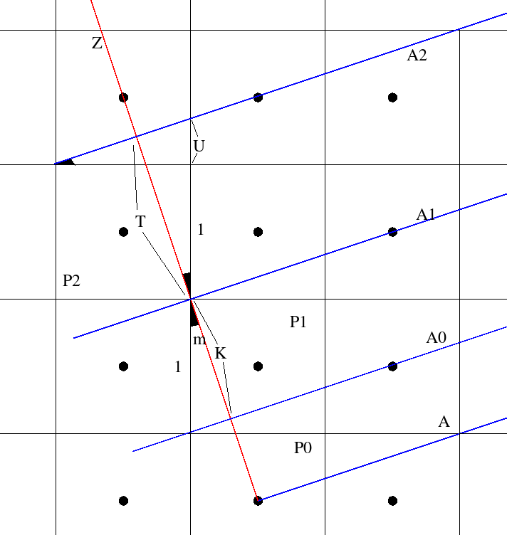
The angle m is the angle of our base line. So
    D= sqrt(dx^2+dy^2)
  tan(m)= dy/dx = U/1    cos(m)= K/1 = T/(U+1) = dx/D

  K= dx/D
  T= dx/D * (dy/dx+1) = dx/D * (dy+dx)/dx = (dy+dx)/D
When we scale these equations with 2D, we get two things:
- We get rid of the floating point numbers.
- The scale matches the scale of the error variables.
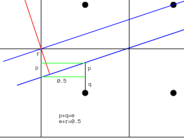
Here, we're interested in the length of the red segment within the pixel. e is the error of the (lower) blue base line. The green lines are parallel to the x axis. Therefore, they form triangles with the base line angle m.
  tan(m)= p/0.5 = dy/dx    p= 0.5dy/dx

  r= 0.5 - e

  p+r= 0.5 - e + 0.5dy/dx

  cos(m)= U/(p+r) = dx/D

  U= dx/D*(0.5 -e + 0.5dy/dx)

  scaled with 2D

   2dx * 0.5 - 2dx*e + 2dx*0.5dy/dx =  dx - 2dx*e + dy
We already know what 2dx*e is: it's the error variable of the base line. For the thickness accumulators in perpendiculars, the initial values and updates are:
          LEFT                            RIGHT
INIT   w= dx+dy-error_A              w= dx+dy+error_A
SQUR   w= w + 2dx                    w= w+2dx
DIAG   w= w + 2dx + 2dy              w= w+2dx+2dy
Interestingly, Murphy doesn't include the term dx+dy for the initial
thickness value. It seems to be getting it wrong for this reason.
When I draw a 45 degree line with width 10, my algorithm draws one
with width 9.9 (7 pixels across). Murphy's algorithm draws the line
with width 11.3 (8 pixels across). Here is the final result of the algorithm.
Below is the final version for octant 1. Main improvements over previous versions are:
- Left and right perpendiculars are collected into one function.
- Proper thickness calculation is done.
perp_octant1(x0,y0,dx,dy,einit,width,winit):

  threshold = dx - 2*dy
  E_diag= -2*dx
  E_square= 2*dy
  wthr= 2*width*sqrt(dx*dx+dy*dy)

  x,y= x0,y0
  error= einit
  tk= dx+dy-winit

  while tk<=wthr:
     pixel(x,y)
     if error > threshold:
       x= x - 1
       error = error + E_diag
       tk= tk + 2*dy
     end
     error = error + E_square
     y= y + 1
     tk= tk + 2*dx
  end

  x,y= x0,y0
  error= -einit
  tk= dx+dy+winit

  while tk<=wthr:
     pixel(x,y)
     if error > threshold:
       x= x + 1
       error = error + E_diag
       tk= tk + 2*dy
     end
     error = error + E_square
     y= y - 1
     tk= tk + 2*dx
  end

thick_octant1(x0,y0,x1,y1,width):

  dx= x1 - x0
  dy= y1 - y0
  p_error= 0
  error= 0
  y= y0
  x= x0
  threshold = dx - 2*dy
  E_diag= -2*dx
  E_square= 2*dy
  length = dx+1

  for p= 1 .. length:
    perp_octant1(x,y, dx, dy, p_error,width,error)
    if error > threshold:
      y= y + 1
      error = error + E_diag
      if p_error > threshold:
        perp_octant1(x,y, dx, dy, p_error+E_diag+E_square,width,error)
        p_error= p_error + E_diag
      end
      p_error= p_error + E_square
    end
    error = error + E_square
    x= x + 1
  end
Without realizing why I did it, I put the second call to perpendicular
after the assignment error= error + E_diag. This is actually
the correct thing to do because at this point, we have moved up one pixel
for the extra perpendicular. The initial thickness to be passed to this
perpendicular should contain the error from moving up, but not the error
from moving right since we're still at the same x coordinate. So this is
accidentally correct.
Handling Other Octants
Let's have a look at our basic Bresenham algorithm:
  error= 0
  y= y0
  for x = x0 .. x1
    pixel(x,y)
    if error + 2dy > dx
      y= y+ 1
      error = error - 2dx
    end
    error= error + 2dy
  end
If we always use non-negative numbers for dx and dy, obviously
the error computation doesn't depend on the direction of the line.
Given non-negative dx and dy, the error code computes a particular sequence of square and diagonal moves. You can use this sequence to move in any of the four directions. For an x-based line our code would look like:
  error= 0
  x,y= x0,y0
  for p= 1 .. dx+1
    pixel(x,y)
    if error + 2dy > dx
      y= y+ ystep
      error = error - 2dx
    end
    error= error + 2dy
    x= x + xstep
  end
By choosing xstep and ystep from {-1,1}, we can make this code paint any x-based
line. The same argument applies to all functions we've written so far. Just
change the increments and you cover the other 3 octants.
For handling y-based lines where abs(dy)>abs(dx), we need a different function because now we're looping over the y coordinates and occasionally updating x coordinates. This could still be stuffed into the same function using even more variables and adding some occasionally-nop code but we will have to sacrifice code readability.
I realized that the line p0->p1 isn't necessarily the same line as p1->p0. The error is defined to be zero for p0. When the code ends, it isn't necessarily zero at p1. The non-zero situation happens whenever dy doesn't divide dx (for octant1). However, it would be zero for p1 if we had switched the points around.
To paraphrase it: the error calculation computes a particular sequence of square and diagonal moves from p0 to p1. This sequence doesn't have to be symmetric. Therefore, if you applied the sequence from p1 to p0, you'd end up with a different set of pixels painted.
Variants
The most powerful aspect of this algorithm is the fact that it can vary the thickness along the base line. This allows drawing very decorative lines. Consider the case where the width function is a sine wave etc. Another possibility is to use this feature to draw lines with perspective. Also, the left and right halves of the line are drawn independently of each other. This allows yet more opportunities to draw decorations.With a minor change to pright_octant1 and its correspondent in perp_octant1, the algorithm can be made to traverse each pixel only once. The only pixels drawn twice are the ones on the base line. This could be eliminated easily. This would allow the algorithm to be used for situations where the objective is not to directly paint but execute some operation on the pixels, such as negating the background, doing an intersection etc.
Since we have a measure of the current thickness in the perpendicular function, we could draw anti-aliased lines using this algorithm. We could vary the brightness as we move away from the center of the thick line.
Implementation
Several of my assumptions turned out to be false when I was doing the implementation. For example, going in reverse on a line is almost identical to going forward, with one crucial difference. In the forward direction, we used error≥threshold to decide for a diagonal. When going in reverse, we need to use error>threshold for diagon decision.Let's say that we're doing the very first example, basic Bresenham line in the first octant. When going forward, the error≥threshold condition selects the upper pixel when error=threshold. When going in reverse from the upper pixel, if error=threshold, we must stay in the upper y coordinate. We should switch to the lower y coordinate when error exceeds threshold. This is necessary because otherwise the left and right sides of a perpendicular get out of phase and artifacts occur.
Another failed assumption was that adapting the code for other octants would be trivial. Not really so. The xstep and ystep values for the perpendiculars have to be chosen carefully such that what I mention as 'left' in this article really follows the normal we've discussed. i.e. the normal coming in from bottom-right to top-left for a line in the first octant.
Actually, trying to go left in the first perpendicular doesn't really work. What we have really discussed in the introduction to perpendicular part is the normal starting from the y-side of the origin and continuing towards to y-side of the target (for an x-based line). This isn't always left. However, I made arrangements in the code such that left and right of a vector are still distinguishable and can be given different thicknesses.
Here is an implementation of the algorithm in this article. There is only one entry function, which takes two functions as arguments. These functions should return the width for the left and right sides. The arguments to these functions are:
- A user pointer.
- The position along the line.
- The total length of the line.
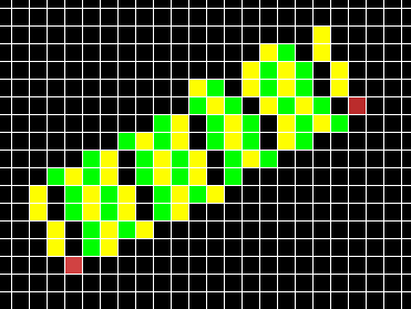
Here are the figures I used,
in case I need to modify them. Below you can see a test run, showing
the different cases I mentioned in the "Variants" section.
The code could be improved in several ways. First of all, there is
no simple fixed-width line drawing function. A wrapper should be
implemented for that.
Secondly, the outer and inner loops aren't in a state suitable for function inlining. The two calls to 'perpendicular' could be reduced to one by playing with the outer loop control a little bit. This would increase the likelyhood of inlining the inner loop since it's a static function called only from one function.
The code I provide here is part of my drawing package I'm working on. You can't compile it out of the box, but adapting it is simple. Simply modify the pbuffer_t* argument to your image type and replace the six calls to 'pixel' accordingly.
Revisit: Anti-Aliasing
Notes
The Multiplication Trick
If there is a control variable X which is always linearly updated, it can be replaced by another variable K if K is maintained to be a constant multiple of X. i.e. we can replace all assignments and comparisions of X with those using K.When doing this, it's very important to initialize K properly. Let's make an example, the basic Bresenham line stuff:
  error= 0
  ..
  if error+dy/dx > 0.5:
    y = y+1
  end
  ..
  error= error + dy/dx
  ..
  error = error + dy/dx - 1
Setting EB= 2dx*error and multiplying everything above with 2dx:
  EB= 0
  ..
  if EB+2dy > dx
    y = y+1
  end
  ..
  EB= EB + 2dy
  ..
  EB = EB + 2dy - 2dx
Then I replace EB with 'error' again.
Links
Here are some links regarding the Bresenham line drawing algorithm:- Program to draw a line using Bresenham's Line Algorithm (BLA)
- The Bresenham Line-Drawing Algorithm
- Bresenham-based supercover line algorithm - paints all the points the line touches.
- Bresenham - Several C functions implementing the Bresenham algorithm for different objects suchs as lines, circles etc.
- Algorithms for drawing thick lines and curves on raster devices
- Murphy's Modified Bresenham Line Drawing Algorithm - The page by Alan Murphy