Sorting Networks
When we want to sort an array of integers, we can transform the problem as follows. Each element in the array has a rank. Let's call this relation R. If R[i]==k, then A[i] is the kTH element in the sorted array A'. So an input array A corresponds to a rank array R, which is simply a permutation of integers 0 to N-1.For a fixed N, can we find an optimum function which makes the minimum number of comparisions to sort N elements?
First we should observe that a comparison between R[i] and R[j] will yield the same result as a comparison between A[i] and A[j]. If we can sort R using this optimum function, then we can sort A in the same way.
To find the optimum function, I could go thru all possible functions and test them with all possible values of R, and then measure which one does best. Here, 'best' could be defined in various ways: average run time, worst run time etc. Instead of going thru all functions, maybe I can go about it in a heuristic way.
When we make a comparision between two elements of R, we're classifying S= megaset of R (all possible values of R) into two classes. For example, let's have 4 elements and we decide to compare elements 0 and 1.
S={
   0: abcd  1: abdc  2: acbd
   3: acdb  4: adcb  5: adbc
   6: bacd  7: badc  8: bcad
   9: bcda 10: bdca 11: bdac
  12: cbad 13: cbda 14: cabd
  15: cadb 16: cdab 17: cdba
  18: dbca 19: dbac 20: dcba
  21: dcab 22: dacb 23: dabc }
The comparison between elements 0 and 1 can result in -1 or 1 (R[0] is
less than R[1] or opposite). We can now partition S into two sets: for the
first one, the comparison results in -1 and for the second one it's 1.
S_01_L= {
   0: abcd  1: abdc  2: acbd
   3: acdb  4: adcb  5: adbc
                     8: bcad
   9: bcda 10: bdca 11: bdac
           16: cdab 17: cdba }
S_01_G={
   6: bacd  7: badc
  12: cbad 13: cbda 14: cabd
  15: cadb
  18: dbca 19: dbac 20: dcba
  21: dcab 22: dacb 23: dabc }
This would be expressed in our function like this:
  if (A[0]<A[1])
  {
    code_01_L
  }
  else
  {
    code_01_G
  }
Now, if we use element 0 again in code_01_L, we will not divide S_01_L
into two equal parts, which we're aiming for. For instance:
S_01_L_02_L= {
   0: abcd  1: abdc  2: acbd
   3: acdb  4: adcb  5: adbc
   9: bcda 10: bdca }
S_01_L_02_G= {
   8: bcad 11: bdac 16: cdab
   17: cdba }
Comparing A[0] to A[2] has now splitted the current set 8:4, which is
not optimum. We made a comparision, but it didn't give us enough information.
Now we have to distinguish between 8 elements within the first set. If we
had made an optimum choice, the comparison would give us exactly one bit
of information and the split would be 6:6. Let's look at the comparison
between element 2 and 3, maybe:
S_01_L_23_L= {
   0: abcd  2: acbd  5: adbc
   8: bcad 11: bdac 16: cdab  }
S_01_L_23_G= {
   1: abdc  3: acdb  4: adcb
   9: bcda 10: bdca 17: cdba }
This is a perfect 6:6 split and should require less operations per
branch.
In our initial comparison 01, instead of partitioning S we could have done a compare-and-exchange operation and transform S into a smaller set like this:
if (A[0]>=A[1]) A[0] <-> A[1];This would transform S into S_01:
S_01= {
   0: abcd  1: abdc  2: acbd
   3: acdb  4: adcb  5: adbc
                     8: bcad
   9: bcda 10: bdca 11: bdac
           16: cdab 17: cdba }
Which is the same thing as S_01_L. After this first exchange, we have
forced A to conform to an element of S_01_L. Now we only need to
distinguish between the members of S_01_L.
It's not clear that we will always have a perfect split. Let's see if that is the case. Now I'll just use the numbers and see where we can go from our current best position S_01_23, which is the result of two perfect splits. We have 6 possible comparisons:
            S_01=       { 0 1 2 3 4 5 8 9 10 11 16 17 }
            S_01_23=    { 0 2 5 8 11 16 }
  01  already done, no effect
  02        S_01_23_02= { 0 2 4 5}
  03        S_01_23_03= { 0 2 5 8 11}
  12        S_01_23_12= { 0 1 6 7 15}
  13        S_01_23_13= { 0 2 8 12}
  23  already done, no effect
So our third comp-ex doesn't help as much, it eliminates 1 or 2 possibilities
from 6 permutations. Maybe my initial choice of 01_23 wasn't so good after all.
Definitely, this requires a search. This was quite obvious when I started
(due to the huge literature about the subject) but I didn't understand
exactly why. I thought maybe
things were getting inefficient because we eventually run into nasty little
sets and
could do better with different splits at the upper levels. It's not so.
Even the upper level sets can't always be partitioned nicely.
I could make a search on this and see which sequence of compare-exchange operations finish the sort fastest. From the Internet, I found this optimal sequence for 4 elements:
            S_01= { 0 1 2 3 4 5 8 9 10 11 16 17 }
         S_01_23= { 0 2 5 8 11 16 }
      S_01_23_02= { 0 2 4 5 }
   S_01_23_02_13= { 0 2 }
S_01_23_02_13_12= { 0 }
Instead of going thru all N! permutations or 2^N bit strings, I thought
maybe I can verify a solution symbolicly? Like this:
 G[0]= A0
 G[1]= A1
 G[2]= A2
 G[3]= A3

    apply (0,1) and (2,3)

 G[0]= min(A0,A1)
 G[1]= max(A0,A1)
 G[2]= min(A2,A3)
 G[3]= max(A2,A3)

    apply (0,2) and (1,3)

 G[0]= min( min(A0,A1), min(A2,A3))
 G[1]= min( max(A0,A1), max(A2,A3))
 G[2]= max( min(A0,A1), min(A2,A3))
 G[3]= max( max(A0,A1), max(A2,A3))

    apply (1,2)
 G[0]= min( min(A0,A1), min(A2,A3))
 G[1]= min(min( max(A0,A1), max(A2,A3)), max( min(A0,A1), min(A2,A3)))
 G[2]= max(min( max(A0,A1), max(A2,A3)), max( min(A0,A1), min(A2,A3)))
 G[3]= max( max(A0,A1), max(A2,A3))
Verifying the 0zix and 3zix elements is straightforward.
 G[0]= min( min(A0,A1), min(A2,A3))= min(A0,A1,A2,A3)
 G[3]= max( max(A0,A1), max(A2,A3))= max(A1,A1,A2,A3)
Obviously, G[2] ≥ G[1] since
  G[1]= min(U,V)
  G[2]= max(U,V)

    so,

  G[0] ≤ G[1] ≤ G[2] ≤ G[3]
I now have the problem of proving that G[i] is unique, resulting in:
G[0] < G[1] < G[2] < G[3]Proving G[0]!=G[3] is trivial, since Ai is unique.
Instead of that, I could name all the intermediate values and establish relations between them.
 step   0    1    2   3    relations
 -----------------------------------
 init   .    .    .   .     -
 01    G1   G2    .   .     G1 < G2
 23    G1   G2   G3   G4    G3 < G4
 02    G5   G2   G6   G4    G5 < G6, G5= min(G1,G3), G6= max(G1,G3)
 13    G5   G7   G6   G8    G7 < G8, G7= min(G2,G4), G8= max(G2,G4)
 12    G5   G9   G10  G8    G9 < G10, G9= min(G7,G6), G10= max(G7,G6)
Going back to the algebraic approach:
order max(a,b) min(max(a,b),c) min(a,c) min(b,c) max(min(a,c),min(b,c))
-----------------------------------------------------------------------
abc      b           b           a       b             b
acb      b           c           a       c             c
bac      a           a           a       b             a
bca      a           c           c       b             c
cab      b           c           c       c             c
cba      a           c           c       c             c

 min( max(a,b), c) == max( min(a,c), min(b,c) )
 max( min(a,b), c) == min( max(a,c), max(b,c) )

Here is the code (base64):

I2luY2x1ZGUgPHN0ZGlvLmg+CiNpbmNsdWRlIDxzdHJpbmcuaD4KI2luY2x1
ZGUgPHN0ZGxpYi5oPgoKCnN0YXRpYyBpbnQgZmFjdFsyMF07CgpjaGFyIE9P
WzIwXTsKCgp2b2lkIGdlbl9tdGhfcGVybShpbnQgTSxpbnQgTixpbnQgKkEp
CnsKICBpbnQgaSxqLGVsdCxpZHg7CiAgc3RhdGljIGludCBmYWN0WzIwXTsK
CiAgaWYgKCFmYWN0WzBdKQogICB7IGZhY3RbMF09IDE7IGZvcihpPTE7aTwy
MDtpKyspIGZhY3RbaV09IGZhY3RbaS0xXSppOyB9CgogIGZvcihpPTA7aTxO
O2krKykgQVtpXT0gaTsKCiAgZm9yKGk9MDtpPE47aSsrKQogIHsKICAgIGlk
eD0gTSAvIGZhY3RbTi1pLTFdOwogICAgZWx0PSBBW2lkeCtpXTsKICAgIGZv
cihqPWlkeCtpO2o+aTtqLS0pIEFbal09IEFbai0xXTsKICAgIEFbaV09IGVs
dDsKICAgIE0gJT0gZmFjdFtOLWktMV07CiAgfQoKfQoKdm9pZCBwcmluYXJy
KGNoYXIgKm1zZyxpbnQgKkEsaW50IE4pCnsKICBpbnQgaTsKICBwcmludGYo
IiVzIixtc2cpOwogIGZvcihpPTA7aTxOO2krKykgcHJpbnRmKCIlYyIsJ2En
K0FbaV0pOwogIHByaW50ZigiXG4iKTsKfQoKaW50IHBlcm1fbnVtYmVyKGlu
dCBOLGludCAqQSkKewogIGludCBNLGksajsKICBNPSAwOwogIGZvcihpPTA7
aTxOO2krKykKICB7CiAgICBNICs9IEFbaV0qZmFjdFtOLWktMV07CiAgICBm
b3Ioaj1pKzE7ajxOO2orKykKICAgICAgaWYgKEFbal0+QVtpXSkgQVtqXS0t
OwogIH0KICByZXR1cm4gTTsKfQoKaW50IG1heChpbnQgeCxpbnQgeSkKewog
IGlmIChzdHJjaHIoT08seCk+c3RyY2hyKE9PLHkpKSByZXR1cm4geDsKICBy
ZXR1cm4geTsKfQoKaW50IG1pbihpbnQgeCxpbnQgeSkKewogIGlmIChzdHJj
aHIoT08seCk8c3RyY2hyKE9PLHkpKSByZXR1cm4geDsKICByZXR1cm4geTsK
fQoKCmludCBtYWluKGludCBhcmdjLGNoYXIgKiphcmd2KQp7CiAgaW50IEFb
MjBdOwogIGludCBOLGksajsKICBpbnQgRj0xOwogIGludCAqUzsKICBpbnQg
YSxiLGM7CgogIE49IDM7CgogIGZhY3RbMF09IDE7IAogIGZvcihpPTE7aTwy
MDtpKyspIAogICAgIGZhY3RbaV09IGZhY3RbaS0xXSppOyAKCiAgYT0gJ2En
OyBiPSAnYic7IGM9ICdjJzsKICBwcmludGYoCiJvcmRlciBtYXgoYSxiKSBt
aW4obWF4KGEsYiksYykgbWluKGEsYykgbWluKGIsYykgbWF4KG1pbihhLGMp
LG1pbihiLGMpKVxuIik7CnByaW50ZigKIi0tLS0tLS0tLS0tLS0tLS0tLS0t
LS0tLS0tLS0tLS0tLS0tLS0tLS0tLS0tLS0tLS0tLS0tLS0tLS0tLS0tLS0t
LS0tLS0tXG4iKTsKICBmb3IoaT0wO2k8NjtpKyspCiAgewogICAgZ2VuX210
aF9wZXJtKGksMyxBKTsKICAgIGZvcihqPTA7ajwzO2orKykgT09bal09ICdh
JyArIEFbal07CiAgICBPT1szXT0gMDsKcHJpbnRmKAoiJXMgICAgICAlYyAg
ICAgICAgICAgJWMgICAgICAgICAgICVjICAgICAgICVjICAgICAgICAgICAg
ICVjICAgICAgICAgIFxuIiwKT08sICAgICBtYXgoYSxiKSxtaW4obWF4KGEs
YiksYyksbWluKGEsYyksbWluKGIsYyksbWF4KG1pbihhLGMpLG1pbihiLGMp
KQopOwogIH0KCiAgcmV0dXJuIDA7Cn0KCgo=

Wait, I like this.

   X=max(a,b)
   Y=min(X,c)
   Z=min(a,c)
   T=min(b,c)
   U=max(Z,T)
order X Y Z T U
---------------
abc   b b a b b
acb   b c a c c
bac   a a a b a
bca   a c c b c
cab   b c c c c
cba   a c c c c


I2luY2x1ZGUgPHN0ZGlvLmg+CiNpbmNsdWRlIDxzdHJpbmcuaD4KI2luY2x1ZGUgPH
N0ZGxpYi5oPgoKCnN0YXRpYyBpbnQgZmFjdFsyMF07CgpjaGFyIE9PWzIwXTsKCgp2
b2lkIGdlbl9tdGhfcGVybShpbnQgTSxpbnQgTixpbnQgKkEpCnsKICBpbnQgaSxqLG
VsdCxpZHg7CiAgc3RhdGljIGludCBmYWN0WzIwXTsKCiAgaWYgKCFmYWN0WzBdKQog
ICB7IGZhY3RbMF09IDE7IGZvcihpPTE7aTwyMDtpKyspIGZhY3RbaV09IGZhY3RbaS
0xXSppOyB9CgogIGZvcihpPTA7aTxOO2krKykgQVtpXT0gaTsKCiAgZm9yKGk9MDtp
PE47aSsrKQogIHsKICAgIGlkeD0gTSAvIGZhY3RbTi1pLTFdOwogICAgZWx0PSBBW2
lkeCtpXTsKICAgIGZvcihqPWlkeCtpO2o+aTtqLS0pIEFbal09IEFbai0xXTsKICAg
IEFbaV09IGVsdDsKICAgIE0gJT0gZmFjdFtOLWktMV07CiAgfQoKfQoKdm9pZCBwcm
luYXJyKGNoYXIgKm1zZyxpbnQgKkEsaW50IE4pCnsKICBpbnQgaTsKICBwcmludGYo
IiVzIixtc2cpOwogIGZvcihpPTA7aTxOO2krKykgcHJpbnRmKCIlYyIsJ2EnK0FbaV
0pOwogIHByaW50ZigiXG4iKTsKfQoKaW50IHBlcm1fbnVtYmVyKGludCBOLGludCAq
QSkKewogIGludCBNLGksajsKICBNPSAwOwogIGZvcihpPTA7aTxOO2krKykKICB7Ci
AgICBNICs9IEFbaV0qZmFjdFtOLWktMV07CiAgICBmb3Ioaj1pKzE7ajxOO2orKykK
ICAgICAgaWYgKEFbal0+QVtpXSkgQVtqXS0tOwogIH0KICByZXR1cm4gTTsKfQoKaW
50IG1heChpbnQgeCxpbnQgeSkKewogIGlmIChzdHJjaHIoT08seCk+c3RyY2hyKE9P
LHkpKSByZXR1cm4geDsKICByZXR1cm4geTsKfQoKaW50IG1pbihpbnQgeCxpbnQgeS
kKewogIGlmIChzdHJjaHIoT08seCk8c3RyY2hyKE9PLHkpKSByZXR1cm4geDsKICBy
ZXR1cm4geTsKfQoKCiNkZWZpbmUgRVFWQVIoWCxZKSBpbnQgWDsKI2RlZmluZSBFUV
NUUihYLFkpICIgIiAjWCAKI2RlZmluZSBFUURFQ0woWCxZKSBwcmludGYoIiAgIiBF
UVNUUihYLFkpICI9IiAjWSAiXG4iICk7CiNkZWZpbmUgRVFMSU4oWCxZKSBlcWxpbi
hFUVNUUihYLFkpKTsKI2RlZmluZSBFUURPKFgsWSkgIFggPSBZOwojZGVmaW5lIEVR
UFJUKFgsWSkgZXFwcnQoWCxFUVNUUihYLFkpKTsKCiNkZWZpbmUgRVFVQVRJT05TIF
wKICBFUShYLG1heChhLGIpKSBcCiAgRVEoWSxtaW4oWCxjKSkgXAogIEVRKFosbWlu
KGEsYykpIFwKICBFUShULG1pbihiLGMpKSBcCiAgRVEoVSxtYXgoWixUKSkgCgp2b2
lkIGVxbGluKGNoYXIgKnRpdGxlKQp7CiAgaW50IGk7CiAgZm9yKGk9MDt0aXRsZVtp
XTtpKyspIHByaW50ZigiLSIpOwp9Cgp2b2lkIGVxcHJ0KGludCB2LCBjaGFyICp0aX
RsZSkKewogIGludCBpOwogIGludCBMPSBzdHJsZW4odGl0bGUpOwogIGZvcihpPTA7
aStpPEw7aSsrKSBwcmludGYoIiAiKTsKICBwcmludGYoIiVjIix2KTsgaSsrOwogIG
Zvcig7aTxMO2krKykgcHJpbnRmKCIgIik7Cn0KCgppbnQgbWFpbihpbnQgYXJnYyxj
aGFyICoqYXJndikKewogIGludCBBWzIwXTsKICBpbnQgTixpLGo7CiAgaW50IGEsYi
xjOwoKICBOPSAzOwoKICBmYWN0WzBdPSAxOyAKICBmb3IoaT0xO2k8MjA7aSsrKSAK
ICAgICBmYWN0W2ldPSBmYWN0W2ktMV0qaTsgCgojZGVmaW5lIEVRIEVRVkFSCiAgRV
FVQVRJT05TCiN1bmRlZiBFUQoKI2RlZmluZSBFUSBFUURFQ0wKICBFUVVBVElPTlMK
I3VuZGVmIEVRCgojZGVmaW5lIEVRIEVRU1RSCiAgcHJpbnRmKCJvcmRlciIgRVFVQV
RJT05TICJcbiIpOwojdW5kZWYgRVEKCiNkZWZpbmUgRVEgRVFMSU4KICBwcmludGYo
Ii0tLS0tIik7IAogIEVRVUFUSU9OUwogIHByaW50ZigiXG4iKTsKI3VuZGVmIEVRCg
ogIGE9ICdhJzsgYj0gJ2InOyBjPSAnYyc7CiAgZm9yKGk9MDtpPDY7aSsrKQogIHsK
ICAgIGdlbl9tdGhfcGVybShpLDMsQSk7CiAgICBmb3Ioaj0wO2o8MztqKyspIE9PW2
pdPSAnYScgKyBBW2pdOwogICAgT09bM109IDA7CiAgICAgICAgICAgIC8vb3JkZXIK
ICAgIHByaW50ZigiJXMgICIsIE9PKTsKI2RlZmluZSBFUSBFUURPCiAgICBFUVVBVE
lPTlMKI3VuZGVmIEVRCgojZGVmaW5lIEVRIEVRUFJUCiAgICBFUVVBVElPTlMKI3Vu
ZGVmIEVRCiAgICBwcmludGYoIlxuIik7CiAgfQoKICByZXR1cm4gMDsKfQoKCg==
So, a new notation is in order to make some manipulations. From now on '.' is minimum and '+' is maximum. '.' may be omitted if unambigous.
 min( max(a,b), c) == max( min(a,c), min(b,c) )

   (a+b)c = ac+bc   // distributive ?? fantastic.

  (a+b)(c+d) = a(c+d) + b(c+d)
             = ac + ad + bc + bd

 G[1]= min(min( max(A0,A1), max(A2,A3)), max( min(A0,A1), min(A2,A3)))
                ----------  ---------           A0.A1         A2.A3
                  (A0+A1)    (A2+A3)
           ----------------------------  ---------------------------
                   (A0+A1)(A2+A3)               (A0.A1 + A2.A3)
                   (A0A2+A0A3+A1A2+A1A3)
      ----------------------------------------------------------------
                   (A0A2+A0A3+A1A2+A1A3) (A0.A1 + A2.A3)

    =  A0.A2.A0.A1 + A0.A2.A2.A3 +
       A0.A3.A0.A1 + A0.A3.A2.A3 +
       A1.A2.A0.A1 + A1.A2.A2.A3 +
       A1.A3.A0.A1 + A1.A3.A2.A3

we have,  X.X= X and Y+Y=Y

    =  A0.A1.A2 + A0.A2.A3 +
       A0.A1.A3 + A0.A2.A3 +
       A0.A1.A2 + A1.A2.A3 +
       A0.A1.A3 + A1.A2.A3

 G[1]=  A0.A1.A2 + A0.A2.A3 + A0.A1.A3 + A1.A2.A3


 G[2]= max(min( max(A0,A1), max(A2,A3)), max( min(A0,A1), min(A2,A3)))
                ----------  ----------        ----------  ----------
                (A0+A1)       (A2+A3)           A0.A1      A2.A3
           ----------------------------  ----------------------------
              (A0.A2+A0.A3+A1.A2+A1.A3)       A0.A1 + A2.A3

      = A0.A2 + A0.A3 + A1.A2 + A1.A3 + A0.A1 + A2.A3

      = A0.A1 + A0.A2 + A0.A3 + A1.A2 + A1.A3 + A2.A3
So, to prove that G[2]≥G[1], we just need to show that max(G[1],G[2]) is
G[2]. This is normally obvious from the fact that one is the minimum
and the other is the maximum of two elements, but I want to develop the
technique. What happens now is that we 'add' (max) the two expressions
together, simplify it, and then see that it's equal to G[2].
  G[1]=  A0.A1.A2 + A0.A2.A3 + A0.A1.A3 + A1.A2.A3
+ G[2]= A0.A1 + A0.A2 + A0.A3 + A1.A2 + A1.A3 + A2.A3
-----------------------------------------------------
        A0.A1.A2 + A0.A2.A3 + A0.A1.A3 + A1.A2.A3 +
        A0.A1 + A0.A2 + A0.A3 + A1.A2 + A1.A3 + A2.A3
It's time to realize more tools for simplification. Obviously,
max(A0.A1+A0.A2, A0.A1.A2) is A0.A1+A0.A2,
but I should prove it somehow.
  a+a.b = a      ... RULE-1

   X=min(a,b)
   Y=max(a,X)
order X Y
---------
ab    a a
ba    b a

  A0.A1+ A0.A2 + A0.A1.A2= A0.A1+ (A0.A2) + (A0.A2).A1
                                  -----as above-------
                         = A0.A1 + A0.A2
In fact, RULE-1 is obvious if you think about the identity elements for
the minimum and maximum operations. Let M be the identity for maximum
and W for minimum. Whenever you find the minimum of W and any a, the
result is a. This means that W is greater than everything else and
similarly M is less than everything else.
  a+a.b = a.W  + a.b
        = a.(W+b)
        = a.W
        = a
I'll go about this in the following fashion. I will keep all expressions
in sum-of-simple-products format, i.e:
G[x]= max( min(elements from Ai), min(elements from Ai), ... )For each min() expression, I will use a machine word. Bit i will be set in the word if Ai occurs in the min() expression. Finally, the whole expression will be a sequence of machine words, terminated by a zero word for convenience.
When I want to find the maximum of two expressions, I simply concatenate them together and simplify the resulting word string. Unifying this string will let me eliminate max(X,X) kind of redundancies. Also, using RULE-1 I will further simplify them.
For finding the minimum of two expressions, I will make a cartesian product of the expressions. The product operation between two machine words will be the bitwise OR operation. This will concatenate the argument lists of the two min() functions, eliminating redundant entries at the same time.
Here it is:
CiNpbmNsdWRlIDxzdGRpby5oPgojaW5jbHVkZSA8c3RkbGliLmg+CiNpbmNsdWRlID
xzdHJpbmcuaD4KCgp0eXBlZGVmIHVuc2lnbmVkIHNob3J0ICB0ZV90OwojZGVmaW5l
IHRlc2l6IHNpemVvZih0ZV90KQoKc2l6ZV90IHRlbGVuKHRlX3QgKlQpCnsKICBzaX
plX3QgaTsKICBmb3IoaT0wO1RbaV07aSsrKSA7CiAgcmV0dXJuIGk7Cn0KCnRlX3Qq
IHRlbmV3KHNpemVfdCBsZW4pCnsKICByZXR1cm4gbWFsbG9jKHRlc2l6KihsZW4rMS
kpOwp9CgppbnQgY29tdGUoY29uc3Qgdm9pZCAqcEEsIGNvbnN0IHZvaWQgKnBCKQp7
CiAgdGVfdCBBLEI7CiAgQT0gKihjb25zdCB0ZV90KilwQTsKICBCPSAqKGNvbnN0IH
RlX3QqKXBCOwogIGlmIChBPkIpIHJldHVybiAxOwogIGlmIChBPEIpIHJldHVybiAt
MTsKICByZXR1cm4gMDsKfQoKc2l6ZV90IHRldW5pZnkodGVfdCAqVCkKewogIHNpem
VfdCBMLGksajsKICBMPSB0ZWxlbihUKTsKICBxc29ydChULCBMLCB0ZXNpeiwgY29t
dGUpOwogIGlmIChMPDIpIHJldHVybiBMOwogIGo9IDA7CiAgZm9yKGk9MTtpPEw7aS
srKQogICAgaWYgKFRbaV0hPVRbal0pCiAgICAgIFRbKytqXT0gVFtpXTsKICBUWysr
al09IDA7CiAgcmV0dXJuIGo7Cn0KCnRlX3QqIHRlc2ltcGxpZnkodGVfdCAqUixzaX
plX3QgbFIpCnsKICBzaXplX3QgaSxqOwogIHNpemVfdCByZW1vdmVkOwoKICBsUj0g
dGV1bmlmeShSKTsKCiAgcmVtb3ZlZD0gMDsKICAgIC8vIFJVTEUtMQogIGZvcihpPT
A7aTxsUi0xO2krKykKICAgIGZvcihqPWkrMTtqPGxSO2orKykKICAgIHsKICAgICAg
dGVfdCBLOwogICAgICBLPSBSW2ldICYgUltqXTsKICAgICAgaWYgKEs9PVJbaV0pIA
ogICAgICB7CiAgICAgICAgIFJbal09IFJbbFItMV07CiAgICAgICAgIGxSLS07CiAg
ICAgICAgIGotLTsKICAgICAgICAgcmVtb3ZlZCsrOwogICAgICAgICBpZiAoaT49bF
ItMSkgZ290byBkb25lOwogICAgICB9CiAgICAgIGVsc2UgaWYgKEs9PVJbal0pCiAg
ICAgIHsKICAgICAgICAgUltpXT0gUltsUi0xXTsKICAgICAgICAgbFItLTsKICAgIC
AgICAgaS0tOwogICAgICAgICBqPSBsUisxOwogICAgICAgICByZW1vdmVkKys7CiAg
ICAgIH0KICAgIH0KZG9uZToKICBSW2xSXT0gMDsKICBpZiAocmVtb3ZlZCkgbFI9IH
RldW5pZnkoUik7CgogIGlmIChyZW1vdmVkPj1sUi8yICYmIHJlbW92ZWQ+PTEwMDAp
CiAgICAgUj0gcmVhbGxvYyhSLCAobFIrMSkqdGVzaXopOwogIHJldHVybiBSOwp9Cg
p0ZV90KiB0ZW1heCh0ZV90ICpBLHRlX3QgKkIpCnsKICB0ZV90ICpSOwogIHNpemVf
dCBsQSwgbEIsbFI7CiAgbEE9IHRlbGVuKEEpOwogIGxCPSB0ZWxlbihCKTsKICBsUj
0gbEErbEI7CiAgUj0gdGVuZXcobFIpOwogIG1lbWNweShSLCBBLCBsQSp0ZXNpeik7
CiAgbWVtY3B5KFIrbEEsIEIsIGxCKnRlc2l6KTsKICBSW2xSXT0gMDsKICByZXR1cm
4gdGVzaW1wbGlmeShSLGxSKTsKfQoKdGVfdCAqdGVtaW4odGVfdCAqQSx0ZV90ICpC
KQp7CiAgdGVfdCAqUjsKICBzaXplX3QgbEEsIGxCLGxSLGksaixrOwogIGxBPSB0ZW
xlbihBKTsKICBsQj0gdGVsZW4oQik7CiAgbFI9IGxBKmxCOwogIFI9IHRlbmV3KGxS
KTsKICBrPSAwOwogIGZvcihpPTA7aTxsQTtpKyspCiAgICBmb3Ioaj0wO2o8bEI7ai
srKQogICAgICBSW2srK10gPSBBW2ldIHwgQltqXTsKICBSW2xSXT0gMDsKICByZXR1
cm4gdGVzaW1wbGlmeShSLGxSKTsKfQoKaW50IHRlY21wKHRlX3QgKkEsdGVfdCAqQi
kKewogIHNpemVfdCBpOwogICAvLyBpZiBCW2ldIGJlY29tZXMgemVybyBiZWZvcmUg
QVtpXSwgQVtpXT5CW2ldIHdpbGwgYmUgdHJ1ZQogICAvLyBhbmQgd2UgcmV0dXJuID
EuCiAgIC8vIGlmIEFbaV0gYmVjb21lcyB6ZXJvIGJlZm9yZSBCW2ldLCB0aGVuIHRo
ZSBsb29wIHN0b3BzCiAgIC8vIGFuZCB3ZSBjaGVjayBmb3IgQltpXS4KICAgLy8gaW
YgdGhleSBib3RoIGJlY29tZSB6ZXJvIGF0IHRoZSBzYW1lIGksIHRoZW4gd2UgcmV0
dXJuIDAuCiAgZm9yKGk9MDtBW2ldO2krKykKICAgIGlmIChBW2ldPEJbaV0pIHJldH
VybiAtMTsKICAgIGVsc2UgaWYgKEFbaV0+QltpXSkgcmV0dXJuIDE7CiAgaWYgKEJb
aV0pIHJldHVybiAtMTsKICByZXR1cm4gMDsKfQoKLy8vLy8vLy8vLy8vLy8vLy8vLy
8vLy8vLy8vLy8vLy8vLy8vLy8vLy8vLy8vLy8vLy8vLy8vLy8vLy8vLy8vLy8vLy8v
Ly8KLy8gTm93IEknbSByZWFkeSB0byBjaGVjayB3aGV0aGVyIHNvbWUgbmV0d29yay
BpcyBhIHZhbGlkIHNvcnRpbmcKLy8gbmV0d29yay4gSSdsbCBidWlsZCB0aGUgZXhw
cmVzc2lvbnMgYXMgSSBkbyB0aGUgY29tcGFyZS1leGNoYW5nZQovLyBvcGVyYXRpb2
5zIGFuZCBjaGVjayB0aGUgb3JkZXIgYXQgdGhlIGVuZC4KLy8gblggaXMgdGhlIG51
bWJlciBvZiBjb21wZXggb3BlcmF0aW9uczogWFsyKmldIGNvbXBleCBYWzIqaV0gCi
8vLy8vLy8vLy8vLy8vLy8vLy8vLy8vLy8vLy8vLy8vLy8vLy8vLy8vLy8vLy8vLy8v
Ly8vLy8vLy8vLy8vLy8vLy8vLy8vCgojaWZkZWYgREVCVUcKdm9pZCBwcmludF9leH
ByKHRlX3QgKlQsaW50IE4pCnsKICBpbnQgaSxqOwogIHRlX3QgSzsKICBmb3IoaT0w
O1RbaV07aSsrKQogIHsKICAgIGludCBjOwogICAgSz0gVFtpXTsKICAgIGM9MDsKIC
AgIGlmIChpKSBwcmludGYoIisiKTsKICAgIGZvcihqPTA7ajxOO2orKykKICAgICBp
ZiAoSyYoMTw8aikpCiAgICAgewogICAgICAgaWYgKGMpIHByaW50ZigiLiIpOwogIC
AgICAgcHJpbnRmKCJhJWQiLGopOwogICAgICAgYz0xOwogICAgIH0KICB9Cn0KCnZv
aWQgcHJpbnRfbmV0d29yayh0ZV90ICoqRyxpbnQgTikKewogIGludCBpOwogIHByaW
50ZigiLS0tLS0tLS0tLS1OZXR3b3JrLS0tLS0tLS0tLS0tLS0tLS1cbiIpOwogIGZv
cihpPTA7aTxOO2krKykKICB7CiAgICBwcmludGYoIkdfJWQ9ICIsaSk7CiAgICBwcm
ludF9leHByKEdbaV0sTik7CiAgICBwcmludGYoIlxuIik7CiAgfQp9CiNlbmRpZgoK
aW50IGlzX3ZhbGlkX3NvcnRpbmdfbmV0d29yayhpbnQgTiwgaW50IG5YLCBpbnQgKl
gpCnsKICB0ZV90ICpHWzIwXTsKICBpbnQgaTsKICBpbnQgUjsKCiAgZm9yKGk9MDtp
PE47aSsrKQogIHsKICAgIEdbaV09IHRlbmV3KDEpOwogICAgR1tpXVswXT0gMTw8aT
sKICAgIEdbaV1bMV09IDA7CiAgfQoKICBmb3IoaT0wO2k8blg7aSsrKQogIHsKICAg
IGludCBMLEg7CiAgICB0ZV90ICpBLCpCOwoKICAgIEw9IFhbMippXTsKICAgIEg9IF
hbMippKzFdOwogICAgaWYgKEw+SCkgeyBMPSBIOyBIPSBYWzIqaV07IH0KCiAgICBB
PSBHW0xdOwogICAgQj0gR1tIXTsKCiAgICBHW0xdPSB0ZW1pbihBLEIpOwogICAgR1
tIXT0gdGVtYXgoQSxCKTsKICAgIGZyZWUoQSk7CiAgICBmcmVlKEIpOwogIH0KCiAg
Uj0gMTsKICBmb3IoaT0xO1IgJiYgaTxOO2krKykKICB7CiAgICB0ZV90ICpNOwogIC
AgTT0gdGVtYXgoR1tpXSwgR1tpLTFdKTsKICAgIGlmICh0ZWNtcChNLEdbaV0pKSBS
PTA7IAogICAgZnJlZShNKTsKICB9CgogIGZvcihpPTA7aTxOO2krKykgZnJlZShHW2
ldKTsKCiAgcmV0dXJuIFI7Cn0KCiNpZmRlZiBTRUxGX1RFU1QKCmludCBtYWluKGlu
dCBhcmdjLGNoYXIgKiphcmd2KQp7CiAgaW50IFhbMTAwXTsKICBpbnQgbngsaSxOOw
oKICBOPSBhdG9pKGFyZ3ZbMV0pOwogIG54PSAwOwogIGZvcihpPTI7aTxhcmdjO2kr
KykKICB7CiAgICBYW254KytdPSBhdG9pKGFyZ3ZbaV0pOwogIH0KICBueC89IDI7Ci
AgcHJpbnRmKCJUaGlzIGlzICVzYSB2YWxpZCBzb3J0aW5nIG5ldHdvcmsuXG4iLAog
ICAgICAgICBpc192YWxpZF9zb3J0aW5nX25ldHdvcmsoTiwgbngsIFgpID8gIiIgOi
Aibm90ICIpOwogIHJldHVybiAwOwp9CiNlbmRpZgoK
So, I made a validator. Later on, I will make some sort of search to pass time.
What the Result Should Look Like
Some notation is in order. The buffers in our network are called G[x,y]. x is the step number and y is the element number. Each step involves only one pair being compexchanged. So the time line for the sorting machine goes like this:
           time / level  -->
 | a   G[0,0]     G[1,0] ...  G[F,0]
 | r   G[0,1]     G[1,1] ...  G[F,1]
 v r   G[0,2]                 G[F,2]
   a   ..
   y   G[0,N-1]   ..          G[F,N-1]
Anyway, let's say that the final array U[z]= G[F,z] for simplicity.
We want to know what U looks like. We already know that the 0zix
element should be the minimum and the last element should be the
maximum of all objects.
  U[0]=   min(A0,A1,..A(N-1))
  U[N-1]= max(A0,A1,..A(N-1))
Also, let's define com(A,z) as the set of z-element combinations of A.
Now, for instance
U[2]= min( x | x= max(a,b,c) | {a,b,c} ∈ com(A,3) )
Let's consider two elements k,e of com(A,3). If max(k) is greater than max(e),
then k can not be the one which goes to the first three elements. Since max(e)
is less than max(k), k contains an element that is larger than all those in
e. When we loop through all elements in com(A,3) in this manner, we reach
the above formula for U[2].
In other words, U[2] is the maximum of three objects. However, it must be the minimum possible to compute in this way.
When we generalize the above formula, we reach:
U[z]= min( x | x= max(v0, v1, .. vz) | {v0,v1,..vz} ∈ com(A,z+1) )
This does generate U[0] properly.
  com(A,1)= { {A0}, {A1} , {A2}, .. {A(N-1)} }

  U[0]= min (max({A0}), max({A1}), max({A2}, ..)
  U[0]= min (A0,        A1,        A2, ..)
It also generates U[N-1]
         has only one element
  com(A,N)= { {A0,A1, A2, .. A(N-1) } }
  U[N-1]= min( max({A0,A1,A2,..}) )
  U[N-1]= max(A0, A1, A2 .. )
Another way to do this is to think about the last p+1 elements of the array
instead of the first z+1, where p+z+1= N.
U[z]= max( x | x = min( {v0,v1,..vp} ) | {v0,v1,..vp} ∈ com(A,p+1) )
Deriving U[N-1]:
  p+z+1= N
  p+N-1= N
  p= 0
  com(A, 1)= { {A0}, {A1}, {A2}, .. }
  U[N-1]= max( min({A0}), min({A1}), min({A2}), .. }
  U[N-1]= max( A0,        A1,        A2 .. )
Deriving U[0]:
  p+z+1= N
  p+0+1= N
  p= N-1
         has one element
  com(A,N)= { {A0,A1,A2, .. } }
  U[0]= max( min({A0,A1,A2,..}) )
  U[0]= min({A0,A1,..})
  U[0]= min(A0,A1,..)
This second form, based on max-of-mins, is more compatible with the way I
implemented expressions before. So, I'm going to use it.
This formula does generate a sorted array. Since the sorted array is unique, all sorting machines should end up with the same expressions for a given N. So, I could verify my findings by trying out the solutions from the internet for various N. Here is the above program with the extra test added:
CiNpbmNsdWRlIDxzdGRpby5oPgojaW5jbHVkZSA8c3RkbGliLmg+CiNpbmNsdWRlIDxzdHJp
bmcuaD4KCgp0eXBlZGVmIHVuc2lnbmVkIHNob3J0ICB0ZV90OwojZGVmaW5lIHRlc2l6IHNp
emVvZih0ZV90KQoKc2l6ZV90IHRlbGVuKHRlX3QgKlQpCnsKICBzaXplX3QgaTsKICBmb3Io
aT0wO1RbaV07aSsrKSA7CiAgcmV0dXJuIGk7Cn0KCnRlX3QqIHRlbmV3KHNpemVfdCBsZW4p
CnsKICByZXR1cm4gbWFsbG9jKHRlc2l6KihsZW4rMSkpOwp9CgppbnQgY29tdGUoY29uc3Qg
dm9pZCAqcEEsIGNvbnN0IHZvaWQgKnBCKQp7CiAgdGVfdCBBLEI7CiAgQT0gKihjb25zdCB0
ZV90KilwQTsKICBCPSAqKGNvbnN0IHRlX3QqKXBCOwogIGlmIChBPkIpIHJldHVybiAxOwog
IGlmIChBPEIpIHJldHVybiAtMTsKICByZXR1cm4gMDsKfQoKc2l6ZV90IHRldW5pZnkodGVf
dCAqVCkKewogIHNpemVfdCBMLGksajsKICBMPSB0ZWxlbihUKTsKICBxc29ydChULCBMLCB0
ZXNpeiwgY29tdGUpOwogIGlmIChMPDIpIHJldHVybiBMOwogIGo9IDA7CiAgZm9yKGk9MTtp
PEw7aSsrKQogICAgaWYgKFRbaV0hPVRbal0pCiAgICAgIFRbKytqXT0gVFtpXTsKICBUWysr
al09IDA7CiAgcmV0dXJuIGo7Cn0KCnRlX3QqIHRlc2ltcGxpZnkodGVfdCAqUixzaXplX3Qg
bFIpCnsKICBzaXplX3QgaSxqOwogIHNpemVfdCByZW1vdmVkOwoKICBsUj0gdGV1bmlmeShS
KTsKCiAgcmVtb3ZlZD0gMDsKICAgIC8vIFJVTEUtMQogIGZvcihpPTA7aTxsUi0xO2krKykK
ICAgIGZvcihqPWkrMTtqPGxSO2orKykKICAgIHsKICAgICAgdGVfdCBLOwogICAgICBLPSBS
W2ldICYgUltqXTsKICAgICAgaWYgKEs9PVJbaV0pIAogICAgICB7CiAgICAgICAgIFJbal09
IFJbbFItMV07CiAgICAgICAgIGxSLS07CiAgICAgICAgIGotLTsKICAgICAgICAgcmVtb3Zl
ZCsrOwogICAgICAgICBpZiAoaT49bFItMSkgZ290byBkb25lOwogICAgICB9CiAgICAgIGVs
c2UgaWYgKEs9PVJbal0pCiAgICAgIHsKICAgICAgICAgUltpXT0gUltsUi0xXTsKICAgICAg
ICAgbFItLTsKICAgICAgICAgaS0tOwogICAgICAgICBqPSBsUisxOwogICAgICAgICByZW1v
dmVkKys7CiAgICAgIH0KICAgIH0KZG9uZToKICBSW2xSXT0gMDsKICBpZiAocmVtb3ZlZCkg
bFI9IHRldW5pZnkoUik7CgogIGlmIChyZW1vdmVkPj1sUi8yICYmIHJlbW92ZWQ+PTEwMDAp
CiAgICAgUj0gcmVhbGxvYyhSLCAobFIrMSkqdGVzaXopOwogIHJldHVybiBSOwp9Cgp0ZV90
KiB0ZW1heCh0ZV90ICpBLHRlX3QgKkIpCnsKICB0ZV90ICpSOwogIHNpemVfdCBsQSwgbEIs
bFI7CiAgbEE9IHRlbGVuKEEpOwogIGxCPSB0ZWxlbihCKTsKICBsUj0gbEErbEI7CiAgUj0g
dGVuZXcobFIpOwogIG1lbWNweShSLCBBLCBsQSp0ZXNpeik7CiAgbWVtY3B5KFIrbEEsIEIs
IGxCKnRlc2l6KTsKICBSW2xSXT0gMDsKICByZXR1cm4gdGVzaW1wbGlmeShSLGxSKTsKfQoK
dGVfdCAqdGVtaW4odGVfdCAqQSx0ZV90ICpCKQp7CiAgdGVfdCAqUjsKICBzaXplX3QgbEEs
IGxCLGxSLGksaixrOwogIGxBPSB0ZWxlbihBKTsKICBsQj0gdGVsZW4oQik7CiAgbFI9IGxB
KmxCOwogIFI9IHRlbmV3KGxSKTsKICBrPSAwOwogIGZvcihpPTA7aTxsQTtpKyspCiAgICBm
b3Ioaj0wO2o8bEI7aisrKQogICAgICBSW2srK10gPSBBW2ldIHwgQltqXTsKICBSW2xSXT0g
MDsKICByZXR1cm4gdGVzaW1wbGlmeShSLGxSKTsKfQoKaW50IHRlY21wKHRlX3QgKkEsdGVf
dCAqQikKewogIHNpemVfdCBpOwogICAvLyBpZiBCW2ldIGJlY29tZXMgemVybyBiZWZvcmUg
QVtpXSwgQVtpXT5CW2ldIHdpbGwgYmUgdHJ1ZQogICAvLyBhbmQgd2UgcmV0dXJuIDEuCiAg
IC8vIGlmIEFbaV0gYmVjb21lcyB6ZXJvIGJlZm9yZSBCW2ldLCB0aGVuIHRoZSBsb29wIHN0
b3BzCiAgIC8vIGFuZCB3ZSBjaGVjayBmb3IgQltpXS4KICAgLy8gaWYgdGhleSBib3RoIGJl
Y29tZSB6ZXJvIGF0IHRoZSBzYW1lIGksIHRoZW4gd2UgcmV0dXJuIDAuCiAgZm9yKGk9MDtB
W2ldO2krKykKICAgIGlmIChBW2ldPEJbaV0pIHJldHVybiAtMTsKICAgIGVsc2UgaWYgKEFb
aV0+QltpXSkgcmV0dXJuIDE7CiAgaWYgKEJbaV0pIHJldHVybiAtMTsKICByZXR1cm4gMDsK
fQoKLy8vLy8vLy8vLy8vLy8vLy8vLy8vLy8vLy8vLy8vLy8vLy8vLy8vLy8vLy8vLy8vLy8v
Ly8vLy8vLy8vLy8vLy8vLy8vLy8KLy8gTm93IEknbSByZWFkeSB0byBjaGVjayB3aGV0aGVy
IHNvbWUgbmV0d29yayBpcyBhIHZhbGlkIHNvcnRpbmcKLy8gbmV0d29yay4gSSdsbCBidWls
ZCB0aGUgZXhwcmVzc2lvbnMgYXMgSSBkbyB0aGUgY29tcGFyZS1leGNoYW5nZQovLyBvcGVy
YXRpb25zIGFuZCBjaGVjayB0aGUgb3JkZXIgYXQgdGhlIGVuZC4KLy8gblggaXMgdGhlIG51
bWJlciBvZiBjb21wZXggb3BlcmF0aW9uczogWFsyKmldIGNvbXBleCBYWzIqaV0gCi8vLy8v
Ly8vLy8vLy8vLy8vLy8vLy8vLy8vLy8vLy8vLy8vLy8vLy8vLy8vLy8vLy8vLy8vLy8vLy8v
Ly8vLy8vLy8vLy8vCgojaWZkZWYgREVCVUcKdm9pZCBwcmludF9leHByKHRlX3QgKlQsaW50
IE4pCnsKICBpbnQgaSxqOwogIHRlX3QgSzsKICBmb3IoaT0wO1RbaV07aSsrKQogIHsKICAg
IGludCBjOwogICAgSz0gVFtpXTsKICAgIGM9MDsKICAgIGlmIChpKSBwcmludGYoIisiKTsK
ICAgIGZvcihqPTA7ajxOO2orKykKICAgICBpZiAoSyYoMTw8aikpCiAgICAgewogICAgICAg
aWYgKGMpIHByaW50ZigiLiIpOwogICAgICAgcHJpbnRmKCJhJWQiLGopOwogICAgICAgYz0x
OwogICAgIH0KICB9Cn0KCnZvaWQgcHJpbnRfbmV0d29yayh0ZV90ICoqRyxpbnQgTikKewog
IGludCBpOwogIHByaW50ZigiLS0tLS0tLS0tLS1OZXR3b3JrLS0tLS0tLS0tLS0tLS0tLS1c
biIpOwogIGZvcihpPTA7aTxOO2krKykKICB7CiAgICBwcmludGYoIkdfJWQ9ICIsaSk7CiAg
ICBwcmludF9leHByKEdbaV0sTik7CiAgICBwcmludGYoIlxuIik7CiAgfQp9CiNlbmRpZgoK
aW50IGZhYyhpbnQgTikKewogc3RhdGljIGludCB0YWJsZVsyMV07CiAgaWYgKCF0YWJsZVsw
XSkKICB7CiAgICBpbnQgaTsKICAgIHRhYmxlWzBdPSAxOwogICAgZm9yKGk9MTtpPDIwO2kr
KykgdGFibGVbaV09IGkqdGFibGVbaS0xXTsKICB9CiByZXR1cm4gdGFibGVbTl07Cn0KCmlu
dCBjb20oaW50IE4saW50IE0pCnsKICByZXR1cm4gZmFjKE4pL2ZhYyhNKS9mYWMoTi1NKTsK
fQoKaW50IHNldF9iaXRzKHVuc2lnbmVkIHNob3J0IGspCnsKICBpbnQgVjsKICBWPSAwOwog
IHdoaWxlKGspCiAgewogICBpZiAoayYxKSBWKys7CiAgIGs+Pj0gMTsKICB9CiAgcmV0dXJu
IFY7Cn0KCmludCBjaGVja19zdHJ1Y3R1cmUoaW50IE4sIHRlX3QgKipHKQp7CiAgaW50IHos
aTsKICBmb3Ioej0wO3o8Tjt6KyspCiAgewogICAgaW50IHAsY29tcHAscHA7CiAgICBwPSBO
LTEtejsKICAgIHBwPSBwKzE7CiAgICBjb21wcD0gY29tKE4scHApOwogICAgaWYgKHRlbGVu
KEdbel0pIT1jb21wcCkgcmV0dXJuIDA7IAogICAgZm9yKGk9MDtpPGNvbXBwO2krKykKICAg
ICAgaWYgKHNldF9iaXRzKEdbel1baV0pIT1wcCkgcmV0dXJuIDA7CiAgfQogIHJldHVybiAx
Owp9CgoKaW50IGlzX3ZhbGlkX3NvcnRpbmdfbmV0d29yayhpbnQgTiwgaW50IG5YLCBpbnQg
KlgpCnsKICB0ZV90ICpHWzIwXTsKICBpbnQgaTsKICBpbnQgUjsKCiAgZm9yKGk9MDtpPE47
aSsrKQogIHsKICAgIEdbaV09IHRlbmV3KDEpOwogICAgR1tpXVswXT0gMTw8aTsKICAgIEdb
aV1bMV09IDA7CiAgfQoKICBmb3IoaT0wO2k8blg7aSsrKQogIHsKICAgIGludCBMLEg7CiAg
ICB0ZV90ICpBLCpCOwoKICAgIEw9IFhbMippXTsKICAgIEg9IFhbMippKzFdOwogICAgaWYg
KEw+SCkgeyBMPSBIOyBIPSBYWzIqaV07IH0KCiAgICBBPSBHW0xdOwogICAgQj0gR1tIXTsK
CiAgICBHW0xdPSB0ZW1pbihBLEIpOwogICAgR1tIXT0gdGVtYXgoQSxCKTsKICAgIGZyZWUo
QSk7CiAgICBmcmVlKEIpOwogIH0KCiAgUj0gMTsKICBmb3IoaT0xO1IgJiYgaTxOO2krKykK
ICB7CiAgICB0ZV90ICpNOwogICAgTT0gdGVtYXgoR1tpXSwgR1tpLTFdKTsKICAgIGlmICh0
ZWNtcChNLEdbaV0pKSBSPTA7IAogICAgZnJlZShNKTsKICB9CgogIFI9IFIgfCAoY2hlY2tf
c3RydWN0dXJlKE4sRykgPDwgMSk7CgogIGZvcihpPTA7aTxOO2krKykgZnJlZShHW2ldKTsK
CiAgcmV0dXJuIFI7Cn0KCiNpZmRlZiBTRUxGX1RFU1QKCmludCBwYXJzZV9hcmcoY2hhciAq
YXJnLGludCAqWCkKewogIGludCBQOwogIGNoYXIgKmVuZDsKICBQPSAwOwogIHdoaWxlKDEp
CiAgewogICAgWFtQXT0gc3RydG9sKGFyZywgJmVuZCwgMTApOwogICAgaWYgKGVuZD09YXJn
KSBicmVhazsKICAgIGFyZz0gZW5kKzE7CiAgICBQKys7CiAgfQogIHJldHVybiBQLzI7Cn0K
CmludCBtYWluKGludCBhcmdjLGNoYXIgKiphcmd2KQp7CiAgaW50IFhbNDAwXTsKICBpbnQg
bngsaSxOOwogIGludCBWVjsKCiAgTj0gYXRvaShhcmd2WzFdKTsKICBueD0gcGFyc2VfYXJn
KGFyZ3ZbMl0sIFgpOwogIFZWPSBpc192YWxpZF9zb3J0aW5nX25ldHdvcmsoTixueCxYKTsK
ICBwcmludGYoIlZhbGlkOiAlc1xuU3RydWN0dXJlZDogJXNcbiIsIFZWJjEgPyAieWVzIiA6
ICJubyIsCiAgICAgICAgICAgICAgICAgICAgICAgICAgICAgICAgICAgICAgICBWViYyID8g
InllcyIgOiAibm8iKTsKICByZXR1cm4gMDsKfQojZW5kaWYKCg==
Here is some input to the program:
 3  0.1/0.2/1.2
 4  0.1/2.3/0.2/1.3/1.2
 5  0.1/3.4/0.2/1.2/0.3/2.3/1.4/1.2/3.4
 6  0.1/1.2/2.3/3.4/4.5/0.1/1.2/2.3/3.4/0.1/1.2/2.3/0.1/1.2/0.1
This looks promising, these sorting machines all conform to my formulas.
I initially thought that symbolic validation would be faster than going thru all cases but it's not so. It's even worse. With the try-and-see approach, we only go thru N! or 2^N cases to see whether the machine sorts. In contrast, the symbolic verification requires us to create expressions with combinatorial size. This requires both time and space proportional to 2^N. However, expressions let me reason about how to search around so I'm going to keep them.
Since I know what the final expressions must look like, I could easily expand the network beyond the input size. For instance, I can have 2N lines for a size N input, copying the input values from [0..N-1] to [N..2N-1]. This would allow me to store intermediate values in the bottom part of the network. At the final stage of construction I could search the array G[0..2N-1] to find the expression for each U[i] and that subset would be my output lines.
In any case, I have the initial and the final states for the G[] network.
 G[0,z]= Az
 G[F,z]= max( min(v0,v1,..vp) | {v0,v1,..vp} ∈ com(A,p+1), p+z+1=N)
Now I need to go from one to the other.
Making a Solution by Hand
In the previous section, I found that thinking about subsets of A is very useful. If I could somehow find relations between min(k) and min(e) where e,k are subsets of A, then I could maybe make a search space out of expressions and then try to find paths from G[0,x] to G[F,x].Let's write out G[F,N-2], the element one before the last.
  say that n= N-1
  G[F,N-2]=  A0.A1 + A0.A2 + A0.A3 ... A0.An +
                     A1.A2 + A1.A3 ... A1.An +
                             A2.A3 ... A2.An +
                                        ...
                                     A(n-1)An
           = A0(A1+A2+...An) +
             A1(A2+A3+...An) +
             A2(A3+A4+...An) +
              ..
             A(n-1)An
I could make a huge circuit for this, and then use the intermediate
results to compute other things.
Let's make one for N=6 and try to reason on it. I'm going to skip the A. On the right side, 0 stands for A0 etc.
  G[F,5]= 0+1+2+3+4+5
  G[F,4]= 0(1+2+3+4+5) + 1(2+3+4+5) + 2(3+4+5) + 3(4+5) + 4.5
  G[F,3]= 0.1.2 + 0.1.3 + 0.1.4 + 0.1.5 +
                  0.2.3 + 0.2.4 + 0.2.5 +
                          0.3.4 + 0.3.5 +
                                  0.4.5
                  1.2.3 + 1.2.4 + 1.2.5 +
                          1.3.4 + 1.3.5 +
                                  1.4.5
                          2.3.4 + 2.3.5 +
                                  2.4.5 +
                                  3.4.5
        = 0.1(2+3+4+5) + 0.2(3+4+5) + 0.3(4+5) + 0.4.5 +
                         1.2(3+4+5) + 1.3(4+5) + 1.4.5 +
                                      2.3(4+5) + 2.4.5 +
                                                 3.4.5

  G[F,2]= 0.1.2.3+ 0.1.2.4+ 0.1.2.5+ 0.1.3.4+ 0.1.3.5+ 0.1.4.5+
                                     0.2.3.4+ 0.2.3.5+ 0.2.4.5+
                                                       0.3.4.5+
                                     1.2.3.4+ 1.2.3.5+ 1.2.4.5+
                                                       1.3.4.5+
                                                       2.3.4.5
        = 0.1.2(3+4+5) + 0.1.3(4+5) + 0.1.4.5 +
                         0.2.3(4+5) + 0.2.4.5 +
                                    + 0.3.4.5 +
                         1.2.3(4+5) + 1.2.4.5 +
                                      1.3.4.5 +
                                      2.3.4.5 +

  G[F,1]= 0.1.2.3.4+ 0.1.2.3.5+ 0.1.2.4.5+
          0.1.3.4.5+ 0.2.3.4.5+ 1.2.3.4.5

        = 0.1.2.3(4+5) + 0.1.2.4.5 +
                         0.1.3.4.5 +
                         0.2.3.4.5 +
                         1.2.3.4.5
  G[F,0]= 0.1.2.3.4.5

Here, the sum A4+A5 and its dual A4.A5 occur very frequently, if we set
     u= A4.A5 and
     U= A4+A5,
maybe we can simplify this a little.


  G[F,5]= 0+1+2+3+4+5 = 0+1+2+3+U

  G[F,4]= 0(1+2+3+4+5) + 1(2+3+4+5) + 2(3+4+5) + 3(4+5) + 4.5
        = 0(1+2+3+U) + 1(2+3+U) + 2(3+U) + 3.U + u

  G[F,3]= 0.1(2+3+4+5) + 0.2(3+4+5) + 0.3(4+5) + 0.4.5 +
                         1.2(3+4+5) + 1.3(4+5) + 1.4.5 +
                                      2.3(4+5) + 2.4.5 +
                                                 3.4.5
        = 0.1(2+3+U) + 0.2(3+U) + 0.3.U + 0.u +
                       1.2(3+U) + 1.3.U + 1.u +
                                  2.3.U + 2.u +
                                          3.u

  G[F,2]= 0.1.2(3+4+5) + 0.1.3(4+5) + 0.1.4.5 +
                         0.2.3(4+5) + 0.2.4.5 +
                                      0.3.4.5 +
                         1.2.3(4+5) + 1.2.4.5 +
                                      1.3.4.5 +
                                      2.3.4.5 +
        = 0.1.2(3+U) + 0.1.3.U + 0.1.u +
                       0.2.3.U + 0.2.u +
                                 0.3.u +
                       1.2.3.U + 1.2.u +
                                 1.3.u +
                                 2.3.u

  G[F,1]= 0.1.2.3(4+5) + 0.1.2.4.5 + 0.1.3.4.5 + 0.2.3.4.5 + 1.2.3.4.5
        = 0.1.2.3.U + 0.1.2.u + 0.1.3.u + 0.2.3.u + 1.2.3.u

  G[F,0]= 0.1.2.3.4.5= 0.1.2.3.u
Now,
      V=3+U and
      v=3.U
seem to be the next best replacement. In order to get rid of the
number 3, I will need yet another one
      x=3.u

  G[F,5]= 0+1+2+3+U= 0+1+2+V

  G[F,4]= 0(1+2+3+U) + 1(2+3+U) + 2(3+U) + 3.U + u
        = 0(1+2+V) + 1(2+V) + 2.V + v + u


  G[F,3]= 0.1(2+3+U) + 0.2(3+U) + 0.3.U + 0.u +
                       1.2(3+U) + 1.3.U + 1.u +
                                  2.3.U + 2.u +
                                          3.u
        = 0.1.(2+V) + 0.2.V + 0.v + 0.u +
                      1.2.V + 1.v + 1.u +
                              2.v + 2.u +
                                      x
        = 0.1.(2+V) + 0.2.V + 1.2.V + (u+v)(0+1+2) + x

 G[F,2] = 0.1.2(3+U) + 0.1.3.U + 0.1.u +
                       0.2.3.U + 0.2.u +
                               + 0.3.u +
                       1.2.3.U + 1.2.u +
                                 1.3.u +
                                 2.3.u
        = 0.1.2.V + 0.1.v + 0.1.u +
                    0.2.v + 0.2.u +
                            0.x +
                    1.2.v + 1.2.u +
                              1.x + 2.x
        = 0.1.2.V + (u+v)(0.1+0.2+1.2) + x(0+1+2)

 G[F,1]= 0.1.2.3.U + 0.1.2.u + 0.1.3.u + 0.2.3.u + 1.2.3.u
       = 0.1.2.v + 0.1.2.u + 0.1.x + 0.2.x+ 1.2.x
       = (u+v)0.1.2 + x(0.1+0.2+1.2)

 G[F,0]= 0.1.2.x

OK. Tidy it up:

 G[F,5]= 0+1+2+V
 G[F,4]= 0(1+2+V) + 1(2+V) + 2.V + v + u
 G[F,3]= 0.1.(2+V) + 0.2.V + 1.2.V + (u+v)(0+1+2) + x
 G[F,2]= 0.1.2.V + (u+v)(0.1+0.2+1.2) + x(0+1+2)
 G[F,1]= (u+v)0.1.2 + x(0.1+0.2+1.2)
 G[F,0]= 0.1.2.x

Some more simplification is due, there are a lot of common factors here

 G[F,5]= 0+1+2+V
 G[F,4]= 0(1+2+V) + 1(2+V) + 2.V + v + u
       = 0.1+0.2+0.V + 1.2 + 1.V + 2.V + (v+u)
       = (0.1+0.2+1.2)+ V(0+1+2) + (v+u)
 G[F,3]= 0.1.(2+V) + 0.2.V + 1.2.V + (u+v)(0+1+2) + x
       = 0.1.2+ V(0.1+0.2.1.2) + (u+v)(0+1+2) + x
 G[F,2]= 0.1.2.V + (u+v)(0.1+0.2+1.2) + x(0+1+2)
 G[F,1]= (u+v)0.1.2 + x(0.1+0.2+1.2)
 G[F,0]= 0.1.2.x

So many things to refactor..
   K= 0.1+0.2+1.2
   L= 0.1.2
   Z= 0+1+2
   M= u+v

 G[F,5]= 0+1+2+V
       = Z+V

 G[F,4]= (0.1+0.2+1.2)+ V(0+1+2) + (v+u)
       = K + V.Z + M
 G[F,3]= 0.1.2+ V(0.1+0.2.1.2) + (u+v)(0+1+2) + x
       = L + V.K + M.Z + x
 G[F,2]= 0.1.2.V + (u+v)(0.1+0.2+1.2) + x(0+1+2)
       = L.V + M.K + x.Z
 G[F,1]= (u+v)0.1.2 + x(0.1+0.2+1.2)
       = M.L + x.K
 G[F,0]= 0.1.2.x
       = L.x

Pretty simple result, it looks like this:
 G[F,5]= Z+V
 G[F,4]= K + V.Z + M
 G[F,3]= L + V.K + M.Z + x
 G[F,2]= L.V + M.K + x.Z
 G[F,1]= M.L + x.K
 G[F,0]= L.x

Now, let's look at what's happening here. K,L and Z are in fact the
resulting of sorting A0,A1,A2. Let's look at the definitions:
   L= 0.1.2                 // minimum of 0,1,2
   K= 0.1+0.2+1.2           // fits perfectly to our formula for the 1zix
                            // element in a 3-element array
   Z= 0+1+2                 // maximum of 0,1,2

The definitions for x,M and V are similar, but there is a little asymmetry
here.
   u= 4.5
   U= 4+5
   M= u+v =  4.5 + 3.4 + 3.5
   x= 3.u =  3.4.5
   V= 3+U =  3+4+5
   v= 3.U =  3(4+5)= 3.4+3.5

again,
   x= 3.4.5             // minimum of 3,4,5
   M= 3.4 + 3.5 + 4.5   // mid element of sort(3,4,5)
   V= 3+4+5             // maximum of 3,4,5
If we wanted to make a circuit out of these, it would look like this:
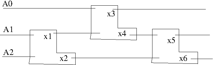
Here the L shaped gates are minmax gates. The upper output is the minimum and the lower output is the maximum for the two inputs on the left.
  x1= A1.A2
  x2= A1+A2
  x3= A0.x1= A0.A1.A2                -> minimum = L
  x4= A0+x1= A0+A1.A2
  x5= x4.x2 = (A0+A1.A2)(A1+A2)
            = A0.A1 + A0.A2+ A1.A2.A1 + A1.A2.A2
            = A0.A1 + A0.A2 + A1.A2  -> mid value= K
  x6= x4+x2 = A0+A1.A2 + A1+ A2
            = A0 + A1 + A2           -> maximum = Z
Now, we can replace these gates with compex operations. This is because
we no longer need the values A0,A1 and A2 for the rest of the computation.
They can simply be replaced by L,K and Z. Also, the size of the circuit
is the same as the number of inputs. This makes it possible to replace
the circuit with a permuting network.
OK. I'm not really confident with my final equations, they look weird. I'll try to derive them again, but doing the replacements from the very start. Here are the new namings:
    a= 0.1.2             d= 3.4.5
    b= 0.1+0.2+1.2       e= 3.4+3.5+4.5
    c= 0+1+2             f= 3+4+5

  G[F,5]= 0+1+2+3+4+5   =  c+f      [FINAL]

  G[F,4]= 0.1+ 0.2+ 0.3+ 0.4+ 0.5+
          1.2+ 1.3+ 1.4+ 1.5+
          2.3+ 2.4+ 2.5+
          3.4+ 3.5+
          4.5
        = b + 0.3 + 0.4 + 0.5 +
               1.3+ 1.4+ 1.5+
          2.3+ 2.4+ 2.5+
          3.4+ 3.5+
          4.5
        = b + 0(3+4+5) + 1(3+4+5) + 2(3+4+5) +
          3.4+ 3.5+
          4.5
        = b + 0.f+1.f+2.f + 3.4 + 3.5 + 4.5
        = b + (0+1+2)f + 3.4+3.5+4.5
        = b + c.f + e
        = c.f + b + e               [FINAL]

  G[F,3]= 0.1.2+ 0.1.3+ 0.1.4+ 0.1.5+
                 0.2.3+ 0.2.4+ 0.2.5+
                        0.3.4+ 0.3.5+
                               0.4.5+
                 1.2.3+ 1.2.4+ 1.2.5+
                        1.3.4+ 1.3.5+
                               1.4.5+
                        2.3.4+ 2.3.5+
                               2.4.5+
                               3.4.5
        = a+d+   0.1.3+ 0.1.4+ 0.1.5+
                 0.2.3+ 0.2.4+ 0.2.5+
                        0.3.4+ 0.3.5+
                               0.4.5+
                 1.2.3+ 1.2.4+ 1.2.5+
                        1.3.4+ 1.3.5+
                               1.4.5+
                        2.3.4+ 2.3.5+
                               2.4.5
        = a+d+   0.1.3+ 0.1.4+ 0.1.5+
                 0.2.3+ 0.2.4+ 0.2.5+
                        0.(3.4+ 3.5+4.5)
                 1.2.3+ 1.2.4+ 1.2.5+
                        1.3.4+ 1.3.5+
                               1.4.5+
                        2.3.4+ 2.3.5+
                               2.4.5
        = a+d+0.e+ 0.1.3+ 0.1.4+ 0.1.5+
                   0.2.3+ 0.2.4+ 0.2.5+
                   1.2.3+ 1.2.4+ 1.2.5+
                          1.3.4+ 1.3.5+
                                 1.4.5+
                          2.3.4+ 2.3.5+
                                 2.4.5
        = a+d+0.e+2.e +
                   0.1.3+ 0.1.4+ 0.1.5+
                   0.2.3+ 0.2.4+ 0.2.5+
                   1.2.3+ 1.2.4+ 1.2.5+
                          1.3.4+ 1.3.5+
                                 1.4.5
        = a+d+0.e+2.e +1.e
                   0.1.3+ 0.1.4+ 0.1.5+
                   0.2.3+ 0.2.4+ 0.2.5+
                   1.2.3+ 1.2.4+ 1.2.5
        = a+d+e.(0+1+2)
                   0.1.3+ 0.1.4+ 0.1.5+
                   0.2.3+ 0.2.4+ 0.2.5+
                   1.2.3+ 1.2.4+ 1.2.5
        = a+d+e.c+
                   0.1.3+ 0.1.4+ 0.1.5+
                   0.2.3+ 0.2.4+ 0.2.5+
                   1.2.3+ 1.2.4+ 1.2.5
        = a+d+e.c+ 3.(0.1+0.2+1.2) +
                          0.1.4+ 0.1.5+
                          0.2.4+ 0.2.5+
                          1.2.4+ 1.2.5
        = a+d+e.c + 3.b + 4.b + 5.b
        = a+d+e.c + (3+4+5).b
        = a+d+e.c + f.b
        = a + b.f + c.e + d         [FINAL]

  G[F,2]= 0.1.2.3+ 0.1.2.4+ 0.1.2.5+
                   0.1.3.4+ 0.1.3.5+
                            0.1.4.5+
                   0.2.3.4+ 0.2.3.5+
                            0.2.4.5+
                            0.3.4.5+
                   1.2.3.4+ 1.2.3.5+
                            1.2.4.5+
                            1.3.4.5+
                            2.3.4.5
        = (0+1+2).3.4.5 +
          0.1.2.3+ 0.1.2.4+ 0.1.2.5+
                   0.1.3.4+ 0.1.3.5+
                            0.1.4.5+
                   0.2.3.4+ 0.2.3.5+
                            0.2.4.5+
                   1.2.3.4+ 1.2.3.5+
                            1.2.4.5
        = c.d+
          0.1.2.3+ 0.1.2.4+ 0.1.2.5+
                   0.1.3.4+ 0.1.3.5+
                            0.1.4.5+
                   0.2.3.4+ 0.2.3.5+
                            0.2.4.5+
                   1.2.3.4+ 1.2.3.5+
                            1.2.4.5
        = c.d+ 0.1.2(3+4+5)+
                   0.1.3.4+ 0.1.3.5+
                            0.1.4.5+
                   0.2.3.4+ 0.2.3.5+
                            0.2.4.5+
                   1.2.3.4+ 1.2.3.5+
                            1.2.4.5
        = c.d+ a.f +
                   0.1.3.4+ 0.1.3.5+
                            0.1.4.5+
                   0.2.3.4+ 0.2.3.5+
                            0.2.4.5+
                   1.2.3.4+ 1.2.3.5+
                            1.2.4.5
       = c.d+a.f+(0.1+0.2+1.2).3.4
                    0.1.3.5+ 0.1.4.5+
                    0.2.3.5+ 0.2.4.5+
                    1.2.3.5+ 1.2.4.5
       = c.d+a.f+b.3.4
                    0.1.3.5+ 0.1.4.5+
                    0.2.3.5+ 0.2.4.5+
                    1.2.3.5+ 1.2.4.5
       = c.d+a.f+b.3.4+b.3.5+
                     0.1.4.5+
                     0.2.4.5+
       = c.d+a.f+b.3.4+b.3.5+b.4.5
       = c.d+a.f+b.(3.4+3.5+4.5)
       = c.d+a.f+b.e
 G[F,2]= a.f + b.e + cd        [FINAL]

 G[F,1]=0.1.2.3.4+ 0.1.2.3.5+ 0.1.2.4.5+
         0.1.3.4.5+ 0.2.3.4.5+ 1.2.3.4.5
       =a.3.4+ a.3.5+ a.4.5++
         0.1.3.4.5+ 0.2.3.4.5+ 1.2.3.4.5
       =a.3.4+ a.3.5+ a.4.5++
         0.1.3.4.5+ 0.2.3.4.5+ 1.2.3.4.5
       = a(3.4+3.5+4.5)+
         0.1.3.4.5+ 0.2.3.4.5+ 1.2.3.4.5
       = a.e +
         0.1.d + 0.2.d + 1.2.d
       = a.e + d(0.1+0.2+1.2)
       = a.e + d.b
       = a.e + b.d              [FINAL]
 G[F,0]= 0.1.2.3.4.5
 G[F,0]= a.d                    [FINAL]
Finally, I got it right this time, I guess:
    a= 0.1.2             d= 3.4.5
    b= 0.1+0.2+1.2       e= 3.4+3.5+4.5
    c= 0+1+2             f= 3+4+5

  G[F,5]= c+f
  G[F,4]= b+cf+e
  G[F,3]= a+bf+ce+d
  G[F,2]= af+be+cd
  G[F,1]= ae+bd
  G[F,0]= ad
Now we need to find terms x,y such that they appear in both x.y and x+y form
in the above equations. When we find them, this means that they are going
to be inputs to a minmax gate and their outputs will be used in the above
formula.
Here are the pairs:
- c and f
- b and e
- a and d
  G[F,5]= c+f
  G[F,4]= b+cf+e
  G[F,3]= a+bf+ce+d
  G[F,2]= af+be+cd
  G[F,1]= ae+bd
  G[F,0]= ad
As you can see above, not all terms are covered by these gates. For example, bf+ce in G[F,3] doesn't include any of our gate outputs. However, maybe we can manipulate these to get better expressions:
  G[F,3]= a+bf+ce+d = a+d + X

  X= bf+ce
             since we know that b<c and e<f,  b= bc and e= ef

  X= bc.f+c.ef = cf(b+e)

  G[F,3]= a+d + cf (b+e)
Done! We expressed G[F,3] in terms of the outputs of our three gates as
described before. Now let's move on to the others
  G[F,2]= af+be+cd
        = be  + af + cd
             we know that a<c and d<f : a= ac , d= df
        = be + ac.f + c.df =  be + cf(a+d)

  G[F,1]= ae+bd
            again, a<b and d<e  so, a=ab and d= de
         =ab.e + b.de  =  be(a+d)
Here are the final results:
  G[F,5]= c+f
  G[F,4]= b+e + cf
  G[F,3]= a+d + cf(b+e)
  G[F,2]= be + cf(a+d)
  G[F,1]= be(a+d)
  G[F,0]= ad
Now we observe that, if we put a,d in a gate and obtain the minimum and maximum results, we will no longer need the values a and d anymore. So, this little gate will act like a small sorting network, replacing the input values. Let's say that
   ad = T     and a+d = U

  G[F,5]= c+f
  G[F,4]= b+e + cf
  G[F,3]= U + cf(b+e)
  G[F,2]= be + cf.U
  G[F,1]= be.U
  G[F,0]= T
The same can be done for other gates as well.
  be= K   and   b+e= L

  G[F,5]= c+f
  G[F,4]= L + cf
  G[F,3]= U + cf.L
  G[F,2]= K + cf.U
  G[F,1]= K.U
  G[F,0]= T
The only remaining pair is cf,
  cf= Y   and   c+f= Z

  G[F,5]= Z
  G[F,4]= L + Y
  G[F,3]= U + Y.L
  G[F,2]= K + Y.U
  G[F,1]= K.U
  G[F,0]= T
So, we can continue constructing our sorting network. We already had two little sorting networks which transformed (A0,A1,A2) to (a,b,c) and (A3,A4,A5) to (d,e,f). I'll start from the output of those:
These three operations don't use each other's values so they can be done in one step.
Here note that T and Z are used in only one place in the equations as the values of G[F,0] and G[F,5]. These are no longer necessary since we have already calculated G[F,0] and G[F,5]. Those lines will continue to the end of the machine, untouched.
We're left with four equations now. Unfortunately, there is no relation between Y and U. Their counterparts have gone outside our scope:
    K<L

  G[F,4]= L + Y
  G[F,3]= U + Y.L
  G[F,2]= K + Y.U
  G[F,1]= K.U
Cheating a Little Bit
I'm stumped with the above equations, I can't figure out which gates I must create to satisfy the equations. Instead, I will simply calculate the two values G[F,4] and G[F,1]. This way, G[x,3] and G[x,2] will end up with some non-derived values which can be simply swapped using a single compex operation. So, the final machine looks like: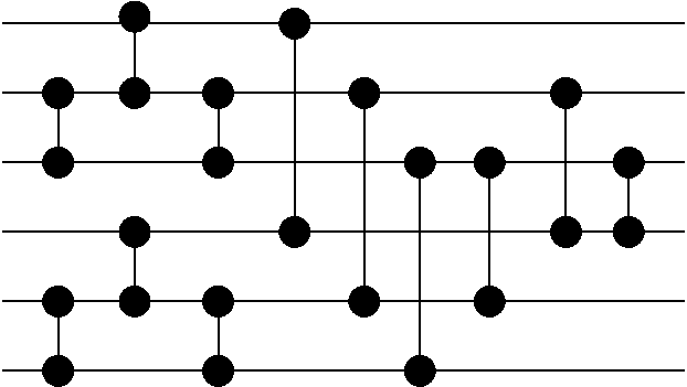
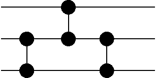
This is 6 levels with 12 comparators. I'll now try this with my validator:
6 1.2/4.5/0.1/3.4/1.2/4.5/0.3/1.4/2.5/2.4/1.3/2.3It does work. How about I try it without the last comparison:
     WARNING: invalid network
  6  1.2/4.5/0.1/3.4/1.2/4.5/0.3/1.4/2.5/2.4/1.3
     WARNING: invalid network
This one didn't work, so I did have to do the last one. Maybe later I'll
try to figure out what exactly got stored in G[F-1,2] and G[F-1,3].
When I got stuck, there wasn't much I could do anyway, I couldn't resolve the situtation with just one level of comparators. So this is indeed the best that could be done in this situation.
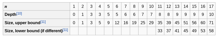
My initial choice of factoring by 3 elements turned out to be poor. According to Wikipedia, my network has one too many layers. I got the number of comparators right. 12 is listed as optimum for 6 inputs.
What Happened Here?
So, I constructed this network in the following manner, I did cheat at the very beginning by immediately jumping to 3-network since I saw a pattern but I paid for it by having one extra level. Maybe if I had started properly according to the following algorithm, I could have ended up with an optimal network, I don't know.First, I wrote down the equations for the final stage of the network. i.e. what do the final values of G[] look like. From there, I tried to find variables x and y such that both x.y and x+y occur in the expressions. These were to be our very first gate inputs.
After that, I used the input variables Ax,Ay to find max(Ax,Ay) and min(Ax,Ay) and then expressed the final values in terms of these values.
By repeating the above process, I reached a point where I couldn't do it any more. At this point, I simply calculated what was easy to calculate and moved on.
The last stages of my construction could be thought of something like a search. However, it's not really a blind search, we have a lot of information about the values in G[x] at that point.
Maybe if I do this right from the beginning, I can end up with slightly better results. Let's do that. Try this with 2 variables at the beginning instead of 3. I did it, and you get stuck much earlier than the 3-variable version.
The problem is that, as you make more and more gates, you lose the symmetry in the equations. This causes some variables to occur many more times than the others and it becomes impossible to derive a clean gate expression from the equations.
Next Steps
There are a couple of avenues I'd like to consider from this point:- Is the reverse of a sorting network also a sorting network?
- Is it possible to move one compex gate to another place and still end up with a sorting network (possibly with less levels)? Naturally, we don't consider moves within the same level; they don't really have an ordering there.
- Some networks are equivalent to each other thru an input rename operation. i.e. if your not-so-sorting network sorts everything else correctly, but the 3rd and the last output are exchanged. In this case, you simply exchange the names of the 3rd and the last lines (you replace their names in the compex gates) and you get a sorting network. Therefore it's sufficient to show that G[F] contains all the necessary final expressions; they can easily be rearranged into the correct order.
Useless Gates?
It's possible to find out whether a given compex gate is useless or not. Here, a gate U: (C,D)= COMPEX(A,B) is useless if A or B can be shown to be equivalent to D. i.e. we know which one is the maximum of A and B just by looking at the expressions describing them.If that is the case, then we don't really need to go thru the gate. The gate can be a NOP or just a shuffle operation. Like this:
 Let  U: (C,D) = COMPEX(A,B)  be our gate, with
    index(A)=index(C)<index(B)=index(D)
 where index(V) is the name of the line. i.e. 0zix line, 1zix line etc.

 if A= MAX(A,B)

   U is a shuffle operation. A and B were already sorted, but in reverse
   order. If we rewrite all compex operations, up to this point, to
   replace A with B and B with A simultaneously, then A and B will
   occur in the correct order at this point of the network. Problem
   solved, we don't need the gate.

 if B= MAX(A,B)

   U is a NOP. We can remove it without any other operation.
Useless gates may or may not occur in algorithmically generated sorting
networks, it's a point to be investigated. However, there is another
application for this.
Let's have a sorting network W. If we prefix this sorting network with a new compex operation U, then the resulting network K=U|W will still be a sorting network. W already sorts its input regardless of how they occur in the input. Adding U doesn't change that fact. Now, we may end up with some useless gates in K-U.
If that is the case, then we can remove the useless gates and potentially may end up with a sorting network with less levels. If there are multiple useless gates, then we have reduced the number of gates which is also good.
Reversal and Reproduction
If the reverse of a sorting network is also a sorting network, then I could have a very fun reproduction operation defined on sorting networks. I could take two parent networks A and B, and then concatenate them (possibly reversing one of them in the process) to get another sorting network C. Now, from there I could eliminate useless gates from C. I'd do this first in the forward direction, and then in the reverse direction. This would let me eliminate gates from both the A-part and B-part of C. In the first run, the first compex of B would be eliminated since A is already a sorting network and anything you do after that is useless. In the second run, something from the A-part of C would be eliminated. It could get interesting.It turns out that the reverse of a sorting network is not always a sorting network. I think I can still create a reproduction operator:
reproduce(A,B):
   C= A + reverse(B)
   loop
     C -= useless(C)
     R  = reverse(C)
     if R is a sorting network
       C = R
   until no useless gates are found
   return C
This operator seems to be asymmetric since the child would probably look
a lot like A rather than B. It's worth a try, but I should first make
a proper network implementation before trying all these new ideas.
The New Operators
So I did try all of that. The prefixing operation is a very good way of generating new sorting networks from existing ones. If a sorting network is doing something stupid like bubbling values up and down, adding a suitable prefix gate can remove multiple gates by the use of the useless gate operator.The useless operator simply looks at the inputs and outputs of each gate and determines whether it's really a NOP. The uselessness of a gate depends on the structure preceding it. So, modifying the beginning of a network will eventually cause some gates in the middle or end of the network to become useless. This doesn't happen so often at the beginning of the network since there isn't enough structure there to make gates redundant.
I have a variation on the useless operator, which also takes into account the structure after the gate in question. It doesn't involve anything fancy, it simply removes a gate from a sorting network and checks whether it still sorts. It's somewhat expensive but it can do things which are hard to prove correct by symbolic manipulation.
There is a variant to the prefixing operation too. If the last level contains a single gate, this is very inefficient. The single gate occupies a whole level by itself and you can't make it more efficient by putting more gates in that level because they will be useless. My rmlast operator tries every possible prefix gate and determines whether adding any of these gates to the start of the network makes that last gate useless. Failing that, it finds the prefix which makes the most number of gates useless. Even if the new prefix gate creates a new level for itself, it still makes sense to do it. The last level is going to be deleted when you find out that the last gate in it is useless. So, the number of levels will still be the same, but we will have a single gate in a level by itself at the beginning of the network rather than the end. The beginning of the network is much more open to manipulation because there is no structure there yet. Almost nothing you add there will be useless.
Another fun one is the 'densify' operator. This one inserts random gates troughout the sorting network. It does this according to these rules:
- The resulting network should still be a sorting network.
- The added gates can not create new levels. They must fit into the levels they were created into.
For densify to work, there should be empty slots in the levels. There we counter the problem of partitioning the network into levels. You can divide a network into levels in many ways, you can agressively pull everything towards one side, as far as they can go, or you can try to balance the levels by minimizing the difference in size between neighbouring levels.
In my implementation I did only two, aggressive pull left and aggressive pull right. These are called normalize and rightnormalize. When you 'normalize' a network, some empty slots will be created at the end of the network. densify then can fill in these slots randomly and make some inefficient gates into useless gates. If you do a rightnormalize, space will open up in the beginning of the network. If you then apply densify in this area, the new gates can affect the rest of the network succeeding them. It's quite hit and miss I can't give a good guideline for this.
I also tried out the reproduction stuff. It does work as I expected but the result is usually worse than what you start with. It has the effect of thinning out the last levels of a network. If it's densely populated by bubble-sort style gates at the end, applying this will remove quite a bit of them at the expense of adding more levels. When you stop the reproduction and cut the network from where it has already sorted the input, the resulting network has more levels at the end than the original one. Needless to say, this operator has very little effect on the beginning of the network.
In my current implementation this operator has some bug which stops me from investigating it further. If I can fix that, maybe it can help thin out the number of the gates at the end, which is a quite difficult task for other operators.
In any case, if you start searching from an already well made network like a mergesort network, it takes a lot of time to reach the optimal solution because the network resists change so much. If you start with a completely random solution or something like bubble sort, then it converges faster and has more chance of getting to the optimum. Here is my current implementation as of 20160725.
Corrections
I made some really stupid mistakes. When I was looking for ways to eliminate the last compex on a level by itself, I constructed candidate networks by prefixing the current network with different gates. Then I looked at useless gates. However there is a much better way: just remove the last gate (or any other gate you want to remove) and add a prefix. When you check whether the network sorts, you're done. It couldn't be any simpler. This will also let me eliminate gates which occupy a level by themselves regardless of where they occur (not just at the last level). This is called 'delsingle' in the implementation below.In addition to this, I fixed the bug in the reproduction operator. repromax does the reproduction as explained previously. It does the flip-remove-useless step as many times as possible. When I was observing it by doing one step at a time, I was under the impression that the operator would thin out the later stages. It's not so. Sometimes it results in very dense stages with almost all slots filled in. It can quickly go from a single gate at the end to a vertical wall.
I also tried to find shuffle gates with no avail. Shuffle gates are similar to useless gates. In useless gates, there is no difference between the input and the output, the inputs arrive at the gate already sorted. In shuffle gates, the inputs arrive sorted in reverse order and this can be shown algebraically. I haven't seen any shuffle gates while I was playing around.
Anyway, I have some operators to work on now, at least. They converge very fast towards the optimum (and also away) but it takes a long time to reach the actual optimum solution. Here is the latest implementation.
More New Ideas
The later stages of networks resist change a lot. In order to overcome this, I can make an operator similar to rmlast or randopfx, but from the other direction. I will add a random gate at the end (without overflowing the level) and then try to remove a gate from the previous levels. If it succeeds, this can be a gain if the removed gate occupied a level by itself. In any case it's good times.Instead of this, now I append a whole vertical wall to the end of the network. A wall is a level which contains compex(2i,2i+1) for all i&leN/2-1. This can remove a lot of gates and potentially merge some levels to recover the level we just added. For this purpose, the operator ScanFwd can be used. This is just like TryDel but scans from the front of the network to the end. Currently, ScanFwd skips the first level and can't remove anything from the front but I will fix that later.
Similarly you can add a wall to the front of the network. This will also create some deletable nodes in the same manner. ScanFwd was in fact created for this operation; try to remove gates except for the ones at the front (we just added them).
In some cases, it's possible to swap two last gates and still end up with a sorting network. Like this for example:
    ----o-------              --------o----
        |                             |
    ----o----o--        to    ---o----o----
             |                   |
    ---------o--              ---o---------
In such a case, I suspect that the middle line is already the mid value
of the three and these two gates are there just to compare the first
and the last lines. If that's the case, then we can replace the whole
thing by one gate. This needs to be investigated.
I did this and found that I was wrong. Even if the swapped network sorts, both gates still have to be present. Since this configuration doesn't resulting in anything being removed, I generalized the swap operation to all gates. The SwapSimple operator swaps two gates at random (which are not in the same level) and checks whether the resulting network sorts. Surprisingly, this operator finds a swappable pair most of the time. Sometimes it has to go thru several iterations but it succeeds still. The effect of this operator is to change the number of levels for a given number of gates. Occasionally it can expose some useless gates if you have too many to start with.
This operator can be used in a search as follows:
  try_swap(N):
    P= swap(N)
    if P.levels < N.levels return P
    return remove_useless(densify(P))
When the search sets a record for number of nodes, I could try doing all
the swaps to see whether there's a network with the same number of nodes
and less number of levels.
Halving a sorting network results in a sorting network for less number of inputs. Sometimes you can even reach the optimum this way. For the converse, I implemented a Double operation. If the number of inputs was N, I first create a network of size 2N. Then I sort two halves using the current network. After that, I sort the middle N values using the current network. Finally, I sort the two N-sized halves using the current network again. The final network sorts if N was even but it doesn't work for odd N. This is understandable. For odd N, the 'middle N' can be determined in two ways and you end up with some unprocessed line whichever you choose.
The third installment of the sorting network tool is here.
Going Back to Generation
Randomly searching around is productive, but generation is more interesting. Maybe it was just luck but I had ended up with the minimum number of gates when I constructed the 6-input network. I want to study this in more depth.This is the plan: I will maintain the expressions for the outputs in my algebraic format. Together with it, I will maintain a relation between input lines. This relation will tell me which line is known to be lesser than which. When I add a gate to the network I'll do two things: rewrite the expressions in terms of the new values and update the relation.
Let's assume that I insert a gate (a,b)=>(a',b') into the network where a'=min(a,b) and b'=max(a,b). I will rewrite each expression in U (the final stage of G[] above). Let's consider the expression U[i]. I'll do the following:
- If a term in U[i] contains a.b, then I'll replace that with a'. We already know that a'=a.b. We're done with this term now.
- If a term doesn't contain a or b, I'll leave it alone.
- I'll list terms which contain a only (from {a,b}) and those with b only. If the intersection of these sets is K, then the sum of the terms in two lists will be K.(a+b)= K.b'. I'll put this in the new expression.
- I'll subtract K from the two lists. If there are remaining elements which contain only a or only b, I don't know how I will resolve it. Maybe I can use some tricks I used above. One option is to abort this gate.
 a'= a.b
 b'= a+b

1:  a' < b'

2:  k<a ∧ k<b ⇒  k<a' ∧ k<b'
3:  k>a ∧ k>b ⇒  k>a' ∧ k>b'

4:  a<k ⇒  a'<k
5:  k<b ⇒  k <b'

6:  k<a ⇒  k ?a' but k <b'
7:  b<k ⇒  b'?k  but a'<k
From the above equations, we can see that the number of entries in the relation will increase by one each time we add a gate. 1: gets added (if a<b was already known, we wouldn't add this gate). 2: thru 5: don't change the relation at all. The last two swap a and b around.
In case the gate is aborted, we can try another. This will constitute a search, which is nice. The nice thing is that, as I add more gates, the final expressions will become simpler, taking up less space. If I can somehow find a way to compress the initial expressions, maybe I can reduce the whole memory requirement by a magnitude. I still don't see how I could make a 64-input network using this but maybe the relation by itself will provide enough information to get by.
Each time I successfully make a gate, I will replace a' by a and b' by b, keeping the number of lines constant. When I do that, I will increase a counter for each a and b, which represents the complexity of the value. When looking for new gates to make, I can combine the least complex values so that the network proceeds in a balanced fashion.
When I get completely stuck, I can fall back to my original trick: just compute whatever is easy to compute and try to recover from that. I could even stop the generation process there and continue with a purely search based approach.
In order to speed up the process, I could even start out with a fixed layer such as a wall. Then, I could generate the final expressions based on the outputs of the wall in the first place, reducing the expression size considerably. It is even possible to do things in parallel. The expressions around the middle of the network are the biggest and they could be split up into chunks, which would be processed in isolation at first.
Some Observations
I have started with this approach. Just like I had experienced, the program gets stuck very early in the derivation of the gates, if limited to my previous tools of factoring.I had designed the ordering relation as a secondary tool to keep track of which lines are less then which lines. However, as I experiment with the program, I realize that the relation is much more useful than I thought especially for rewriting the final expressions.
In my manual generation effort, I had used the following simple rules for rewriting the final expressions. I implemented these in the program, and was able to deduce one further rule. Here are the simple ones:
Let us make a gate (a,b) => (a',b') and C be a term (minimum of some elements) which doesn't contain a or b. We then can rewrite:
After renaming, these two expressions become C.a and C.b respectively.Now I have thought of a new rule, let's look at it:
We have
   C.x.b       where  x < a according to R

we can rewrite this as:

   C.x.a.b     since   x = x.a  (because x<a)

this is equal to:

   C.x.a'

and after renaming:

   C.x.a    ( this a is not the same thing as the previous
              a. this one is the value of a after the gate
              has finished running).

Let's think about this:
         x.b   a'   x.a'
         --------------
  x<a<b   x    a     x     [[ since x<a and a<b => x<b ]]
  x<b<a   x    b     x
  b<x<a   b    b     b
I will call this RULE-4. The same thing applies to C.x.a:
We have

   C.x.a     x < b

 C.x.a =  C.x.b.a = C.x.a'

  after renaming, it's C.x.a again.
Let's call this RULE-5 in the code.
OK one more rule (RULE-6). This was actually something I had used when I was manually building a sorting network. The idea is to find a common factor between two terms and combine them, just like I did for the simple RULE-3. In this case, the common factor doesn't occur naturally inside the two terms. It has to be derived from the terms by adding redundant elements.
  rule6(C.a, D.b, a, b)
    F= maximize(C.a)
    G= maximize(D.b)
    R= F & G
    if  R contains C and D, then rewrite C.a+D.b as  R.b'
    This is called R.b after renaming.
Consider the following case:
Ordering Relation

  012345
 0.<<...
 1>.....
 2>.....
 3....<<
 4...>..
 5...>..

rewriting for gate(0,3): 04+13

Here, neither 04 nor 13 can be rewritten using previous techniques.
However, we can do the following according to RULE-6:

  04 = 014     13= 134
  04+13=  014 + 134 =  14(0+3)  = 14.3'
It's worth noting that R should be reduced to its minimum, in order to avoid making expressions bigger than they need to be.
When applied to a partial expression, I will try all pairs of terms in order. When two terms get combined like this, I will record the result and mark both terms as removable. However, I won't actually remove them from the expression since one term may combine with two or more terms and might be needed later.
After all terms are processed in this way I remove the ones marked as removable.
Another transformation I apply to expresssions is as follows:
  if E = A + B + C   and   B > A,

    then E= B + C
This is called RULE-8. Finding out whether a complex
term B is greater than A is not trivial. I do it in the following way:
- Let A = a0.a1...an
- Let B = b0.b1...bm
- For bj, if there is some ai such that bj>ai, then we can append bj to A without changing its meaning, i.e. A' = A.bj = A
- If bj is included in A, then we don't need to find some such ai, since we can still append bj to A without affecting its meaning.
- When you do the above for all bj, then we will have A' = A.B = A.
- By RULE-1, B + A.B = B.
Right now the program is in a state similar to a manual-search engine. There is no backtracking but all candidate gates are considered until I find a successful one.
If I make a search based on this algebraic approach, two factors will affect the space searched and the order it's searched. First, the set of simplification rules will determine which gates can be created from analysing the final expressions. As you add more rules, the final expressions become simpler. These simpler expressions lend themselves more easily to creation of gates when compared to more complicated expressions.
Second, the order in which the candidate gates are tried affects the order the space is searched. I've tried a couple of criteria for this. If I prioritize gates for which the distance between the inputs is smallest, the program ends up with bubble sort. If I do the reverse, but also insist that the inputs be of the lowest complexity (has gone thru minimal number of gates so far), then the program creates the beginnings of merge sort, but then deviates.
Even the algorithm used for sorting the candidate gates affects the results. An unstable sort seems to do better because a stable one will leave the candidate gates in the order it finds them and that tends to concentrate the effort on the top side of the network, leaving the rest mostly unmodified. This quickly results in irreducible final expressions.
The sorting criteria for candidate gates could be varied as the network progresses. I could first favor gates with distant input lines and then switch to favoring gates near the edges etc.
Where to Go From Here
The current set of rules are pretty good up to N=10. They find sorting networks with almost optimum size without even trying. For example, I was stuck when trying to finish off my hand made 6-input network. I gave the same position in the network to the program and it was able to find out the remaining gates. It couldn't deal with the first replacements which involved three variables each, but I made suitable 3-sorters for the program.Doing a search using the expressions as a guide seems pretty reasonable, but it would be quite slow since each gate entails a lot of rewriting work. Even if I make a much larger set of simplification rules, a search is mandatory because often the networks created have too many levels. Up to 8 inputs, the output has optimal size, but the program overshoots by one gate for 9 inputs. I haven't solved the 10 input case with it, this requires backtracking.
The relation also contains a lot of information. Most of this information isn't available from the expressions themselves because the expressions in the network or in the outputs get transformed radically with each gate. Processing them algebraically without the aid of the relation becomes more and more fruitless as they get simpler. Maybe it could be a good idea to perform a search using the relation as the only guide. I could forgo the whole algebraic system and proceed with the entries in the relation only.
Here is an open question, QUESTION-1. Starting from an empty network and an empty relation, if we apply a sequence of gates to the relation according to RELATRAN and end up with a full relation, does the sequence of gates necessarily form a sorting network? I have suspicion that not-sorting networks would also create full relations occasionally. If that wasn't the case then verifying that a network sorts would become a polynomial problem rather than an exponential one and somebody would have found it by now. This is still worth consideration, maybe I could enumerate all networks which end up with a full relation and see if any of them doesn't sort, for small N of course, like 5 or 6.
So, first thing is to make a backtracking search program based on the relation only. I will use the expression based verifier. Initially, I will use the search program to find ALL networks with full relations, just to progress the above idea. Later on, I'll use pruning to skip over things when they have too many gates/layers. In any case, here is the latest version with all the algebraic tricks.
Searching Based on Relation Only
This idea works, to some extent. The relation keeps a lot of information around but loses some occasionally. There seems to be a limit to how many gates the technique must use to construct a sorting network. Since it loses some information, it creates some unnecessary gates. The fact that these gates are unnecessary can only be found by trial and error. The lost information probably encodes something like a<max(b,c) etc, which become relevant later in the network.Let's look at an example: For 5 inputs, the program creates a network with 10 gates. After that, it can't find anything shorter and exhausts the search space. Quite unusual. When I later apply the TryDel operator I discussed above, I find a deletable gate. Depending on the way I sort gate candidates, I end up with different sorting networks with the same number of gates. Some of these networks can be processed by TryDel to achieve an optimal sized network. Some don't. When I find an M-sized network, I skip all other networks that are longer than or equal to M-gates. This is the reason why I can't find such an optimizable network every time I change the ordering of the candidate gates.
In any case, search using only the relation isn't very productive, but there is a positive outcome. It seems that the answer to QUESTION-1 is "Yes?". Up to 11 inputs I never found any network which provides a full relation but doesn't sort. At 16 inputs I got one but I have doubts about the verifier because the expressions get quite large and I might have some memory issues there. It just seems obvious that a full relation should imply a sorting network but I need to prove it before I can use it as a verifier. I still have doubts, if it was this simple somebody would have thought of it by now. There must be something I'm missing. Maybe the 16-input case was correctly identified? I don't know I should look into this.
Update: I found a bug in the verifier. I wasn't computing number of combinations correctly for N≥13 because the factorials overflowed. Now I do it with proper factorization etc. and it seems that the answer to QUEST-1 is more likely to be YES. I have run the program with different number of inputs for quite some time and haven't seen any network where the relation is full but the network doesn't sort. This update isn't included in sor5 below.
Since searching by relation only isn't very productive, I have to go back to my algebraic approach. In the manual search using the algebraic approach, I had one more algorithm which I didn't mention. After forming a gate, I look at the expressions in the network (not the final expressions) to find out which line is less than which line. By doing these manipulations, I was able to find out more entries for the relation. I just made a test with 6 inputs and found that 12 entries in the relation were recovered in this way. Keeping a network is somewhat expensive because the expressions in it become more and more complicated as the network progresses. However, this might be the only way to move forward.
The relation-only search program is here. I have another idea for this avenue. It's highly unlikely to yield anything but I could give it a try if run out of options. Instead of overwriting elements a and b, I could append new elements a' and b' into the relation and keep a and b as is. Maybe this could eliminate some of the information loss.
Going Back to The Very Beginning
I was looking at how comparators could partition the set of permutations. I could do the same with 2^N bit strings. This could be fun.
  S= {  0: 0000   1: 0001  2: 0010  3: 0011
        4: 0100   5: 0101  6: 0110  7: 0111
        8: 1000   9: 1001 10: 1010 11: 1011
       12: 1100  13: 1101 14: 1110 15: 1111 }

 S_01=             { 0, 1, 3, 4, 5, 7, 8, 9, 11, 12, 13, 15 }
 S_01_23=          { 0, 1, 3, 4, 5, 7, 12, 13, 15 }
 S_01_23_02=       { 0, 1, 3, 5, 7, 9, 13, 15 }
 S_01_23_02_13=    { 0, 1, 3, 5, 7, 15 }
 S_01_23_02_13_12= { 0, 1, 3, 7, 15 }
The result is interesting. It consists of words of type 0K1N-K. Let's do a non-optimal move at some point:
S_01_23_02_03= { 0, 1, 3, 5, 7, 9, 13, 15 }
OK. It looks like I messed up doing it manually. Here is the real run
for the optimal network:
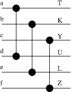
0 1 2 3 4 5 6 7 8 9 10 11 12 13 14 15
0 1
0 2 3 4 6 7 8 10 11 12 14 15
2 3
0 2 3 8 10 11 12 14 15
0 2
0 2 6 8 10 12 14 15
1 3
0 8 10 12 14 15
1 2
0 8 12 14 15
-1 -1
0000
1000
1100
1110
1111
After we got S_01_23_02, we could do the following moves: 01, 02, 03, 12, 13, 23.Let's look at all these:
  S_01_23_02   = 0  2  6  8 10 12 14 15

  S_01_23_02_01= 0  2  6  8 10 12 14 15
  S_01_23_02_02= 0  2  6  8 10 12 14 15
  S_01_23_02_03= 0  2  6  8 10 12 14 15
  S_01_23_02_12= 0  4  6  8 12 14 15
  S_01_23_02_13= 0  8 10 12 14 15
  S_01_23_02_23= 0  2  8 10 12 14 15
Here, the optimal gate stands out very nicely. Some gates are seemingly useless and the other sub-optimal ones reduce the set less. I wonder if this could be carried on to higher number of inputs.
The ordering relation looks like the following after we reach S_01_23_02:
  0123
 0.<<<
 1>...
 2>...
 3>...
The uselessness of the gates involving input 0 is obvious from the relation.
Now I'm thinking of making a search based on this. I will use the relation as the guide again but this time, I'm hoping that useless gates will be found immediately and their subtrees will not be searched.
Now I have a new open question: QUESTION-2.
If a candidate gate (a,b) doesn't modify any of the input values, can we insert a<b into R?Anyway, back to the augmented search. The search will be guided by the partial ordering relation but as I add gates, I will also compute the set of input integers after the gate. For instance, after the gate 01, no input values will have 1 for the 0zix bit and 0 for the 1zix bit. So, the possible values for this pair will be 00, 10 and 11.
If I start the network with a vertical wall, these values will apply to all pairs within the wall. Therefore, I will have only 3^8=6561 different input values past the wall for 16 input lines. I can even use this for verification, which will be much faster.
Results
I did the above. The new program is just another iteration of the relation-only search, with the input set stuff added. I basicly use the size of the input set resulting from a given gate as the metric for that gate. I also update the relation based on findings from the input sets. This results in much better ordering of candidates.It turns out that my pruning implementation for level permutations was incorrect. When I turned that off, the search finds optimum networks for 5,6 and 8 inputs almost instantly. For 7 inputs, it gets stuck at 17 gates 7 levels for a long time. I didn't continue searching further.
The networks found for 6 and 8 inputs are interesting. They are composed of optimum sub-networks, followed by some merging network. In fact, the 8 input network is completely symmetric with regards to the middle line of the network, drawn horizontally. The only starting gates were that of a wall. Now I wonder if I could start with two optimal sub-networks and then search for the merging part only. This would reduce the number of valid inputs past the starting condition even further.
If we had 16 inputs, we would divide it into two halves of 8 inputs each. These have 9 distinct outputs. So, the start of the merging network would have only 9*9=81 input values. This would make for a super fast verifier.
Also, the answer to QUESTION-2 seems to be YES. I did insert the mentioned ordering into the relation when I saw the condition and it didn't break anything. Typically, when I do something unproven, it results in a lot of networks which should sort but don't. In this case, this never happened in the area I covered. Of course this needs further investigation but I can use it for now.
Here is the 6th installment, 15 September 2016.
Next Steps
Let's look at the facts. Searching solely on the relation can't find optimum networks. RELATRAN can't capture all the available information, so it can't identify sorting networks near the optimum. As I understand it, not all sorting networks result in a full relation if we only use RELATRAN.Given some fixed gates at the beginning, we can reduce the number of necessary input sequences to test. This results in a very fast verifier. I have implemented one case of fixed gates: a vertical wall. Another case is the combination of two optimal sub-networks.
So, maybe it's time I give up completely on algebra based networks. The input set based verifier can be used just as effectively, provided that I prefix the network with some gates. Even if the prefix is empty, the worst case is the same as the algebra based verifier: 2N space and time.
I implemented a new prefix for search: subnet. The input lines are divided into half and each half is sorted by a known optimal network. After that, I search for the rest of the network. This has yielded a very nice result for 7 inputs. For larger input values, this typically approaches the optimum faster, but still requires a lot of search to actually get there. For instance, the 8-input problem finds the optimum solution almost immediately when starting from a wall. However, it struggles to get there with this new prefix. This is interesting because the wall-based solution already contains two 4-sorters at the very beginning.
My previous algorithm for pruning permutations within each level was incorrect and skipped over many legitimate areas to search. Therefore, it failed to find the optimum solutions. I have a new one. When I add a gate to the network, I check whether this one forms a new level. If so, I continue with the search. Otherwise, I check whether the gates in the level are sorted according to their upper input line. If not, then I abort this gate because the current level is just another permutation of something we already saw or will see. In this check, I don't include the first gate in a level because if we allow the first gate to change, then the level allocation for the whole network could change, making it impossible to reach some configurations.
In any case, currently I'm searching K different orderings for each level. Without this pruning I was searching K! orderings. This is quite a speed up if not perfect. The program exhausts the 7-input search space, prefixed with subnets, in a very short time. For others the effect isn't so visible.
The latest program is here, dated 19 September 2016.
Another Approach
I've observed the following for a long time, but I hadn't tested its effects on optimal networks:If you remove the top or bottom line (or both) from a sorting network, the result is also a sorting network.This is quite obvious: just assume that you feed the original network with an element less than every other value possible at position 0. The 0zix element would never move and the rest would become sorted since the network sorts EVERYTHING. If you now simply remove the first line, then the rest of the network is still a sorting network.
When you apply this to an optimal sorting network, a strange thing happens: the result is also optimal, after removing useless gates. I verified this from 8 down. The thing is, although an optimal network reduces to another optimal network, the reverse isn't necessarily true. If I start with a random optimal network for N inputs, I can't be sure that I'll end up with an optimal network for N+1 inputs if I simply add gates to it. Maybe the ones which give this result are in a seperate class of optimal networks.
So, here is the new deal: I will try to find an optimal network by adding a new line to a lesser network. This will require me to do a search on all levels. i.e. the network no longer changes only at the end, but everywhere. In order to do this efficiently, I should implement my inputset based verifier.
Results
The inputset based verifier works, I no longer use the algebraic one but it's still in the code. For the new verifier to be more efficient than the old one, the first level needs to be pretty full. If you have a network similar to (0,1) (0,2) (0,3) .. (0,N-1) (1,2) (1,3) .. the new verifier will perform even worse than the old one.I was too quick to generalize my observation above. If start with a random optimal network, removing the top or bottom of the network doesn't necessarily form another optimal network. The reverse isn't true either. If you start with a random optimal network, add an input line but limit the depth of the network, you aren't even guaranteed to find a sorting network, let alone an optimal one. Here is the 8th version implementing this idea.
I've found that even though adding one line to an optimal network may not yield useful results, adding two lines sometimes does. However, this results in a much larger search space, especially if I also add a level in the process. This search takes too long, going thru all networks is just not feasible. So I have to prune by gate numbers here also.
The current method of generating levels is fine, but adding pruning into there might be problematic because it's already quite complicated. So, I need a new way of generating the subsets. I think I should also prune useless gates, it will cut down a lot of search time. I could use my relation technique for this. Although incomplete, it provides quite a bit of information. When you find out that a gate is useless (thru processing the input for it) and then add that information to the relation, then the relation also has full information (enough to be a verifier).
So here is my dilemma, if I make a level-based search I can skip all the permutations of the level. This is a must and I can't go back. However, the relation works on a gate-by-gate basis. I have to somehow generate the levels consistent with both models. Instead of simply storing numbers for gates, I could make more complicated data structures for them which could hold the relation stuff also. When I add the relations, the levels become dependent on each other since now they affect each others valid search space. This is good but complicates the search. I think the best way to go about this would be to incrementally generate all combinations for a level when a previous level changes. So, here is the new idea:
If we have a network of levels L0, L1, .. Lm, then we proceed as follows.
- Step Lm and check for sorting network.
- If Lm can't be stepped any more, step L(m-1) and reset Lm accordingly.
- If L(m-1) can't be stepped either, go back and step L(m-2).
- If you go back as far as L0 and can't step any more, search has ended.
- If you are able to step at any Lk, then init L(k+1) .. L(m) accordingly.
- Each level will be an array of gate objects.
- Each gate object will contain the relation resulting from the execution of the gate.
- If we have gates A,B,C,D,E available they will be used in the
following order, assuming a maximum count of 3:
- A, AB, ABC, ABD, ABE, AC, ACD, ACE, AD, ADE, AE,
- B, BC, BCD, BCE, BD, BDE, BE,
- C, CD, CDE, CE,
- D, DE
- When I decide to go forward with a gate list for the level, I will compute the linelist resulting from it. If I find that the last gate is useless, then I will abandon this gate list as well as all super-sequences. For instance, if I find out that 'B' is useless when trying to proceed with 'AB', then all the subtree starting with AB (ABC, ABD, ABE etc) will be cancelled.
- The maximum count for a level will be determined from the
limit for the search.
ngates(L)= number of gates for level L nfixed(L)= number of fixed gates for level L maxcount(Li)= limit - ngates(0) .. - ngates(L(i-1)) - nfixed(Li) .. - nfixed(Lm) - I don't think I will ever see this, but if a fixed gate turns out to be useless, then I abandon this level completely and go back one level. I'm interested only in networks which contain the initial state. If I started modifying fixed gates, then this would deteriorate to a full-space search, which I'm trying to avoid here.
So, here is my new level generator algorithm:
- The main operation is the addition of a gate to the level.
- This will fail occasionally, for two reasons:
- I might have run out of gates to choose from.
- I might reach the maximum count for the level.
- When such a failure occurs, I move the last element forward.
- If this fails also, I will remove the last element and try to move the previous element forward.
List of Known Optimum Sizes