Detecting a Ball
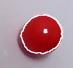
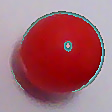
I'm making a robot which will navigate using some artificial landmarks. These landmarks will include some solid color balls. In order to find the landmark, I need to detect these balls. I will use the following image as an example scene, a ball to taped to a cupboard: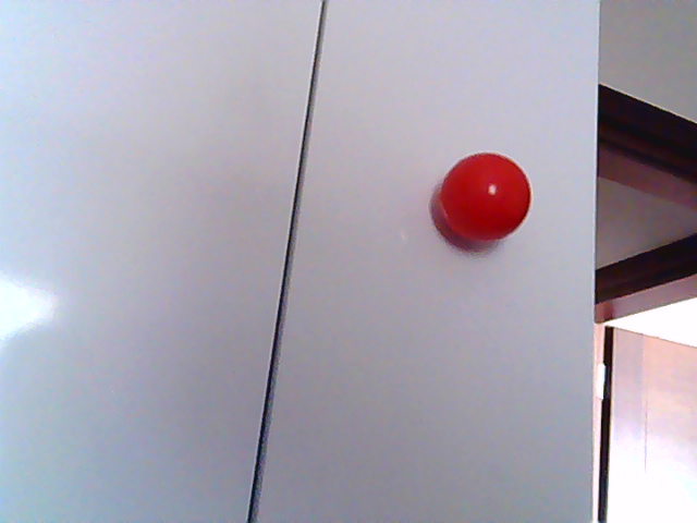
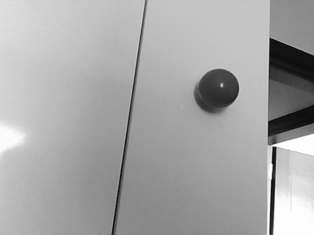
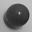
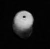
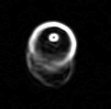
 [G1]   gray=  1.8*RED - 0.9*GREEN - 0.5*BLUE
 [G2]   gray=  0.3*RED + 0.6*GREEN + 0.1*BLUE
G2 is widely used for greyscale conversion. It captures changes in luminosity very well but loses color information. Here is its result:
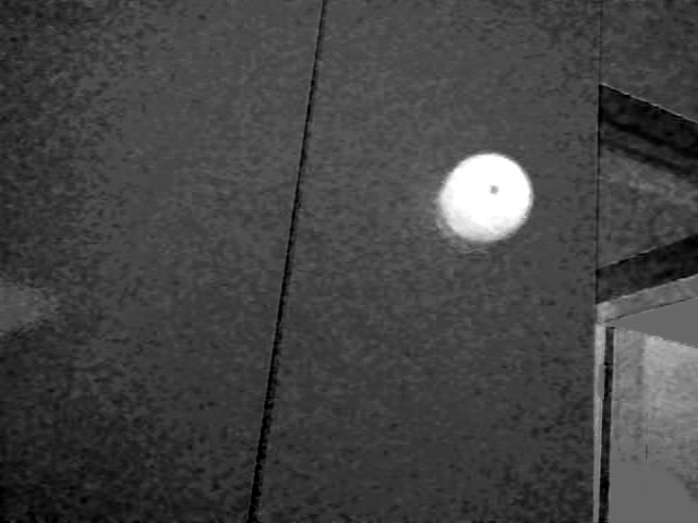
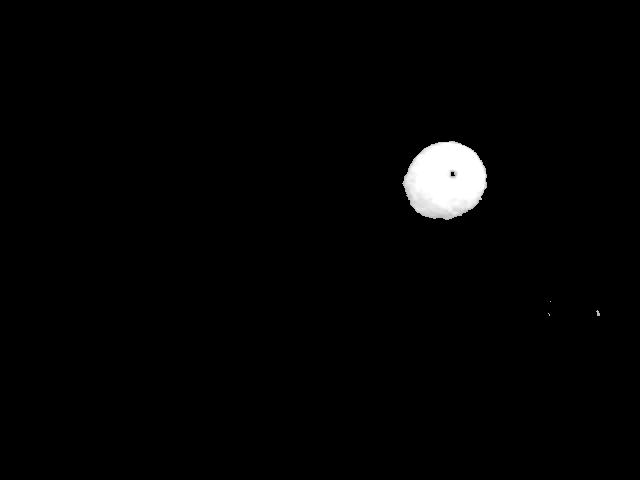
In any case, it's obvious that I can't use t3 or t4 as my base image. I can use t4 as a mask in order to eliminate most of the image in order to speed up the process.
Determining Area of Interest
I will implement a very simple algorithm for this. I will simply divide the image into NxN blocks and find the average pixel value within each block. If the average is above a certain level, then I will conclude that the pixel block has valuable data. Otherwise, it will be ignored. I will then cut the image to the smallest size (plus a small margin on each side) where it contains all valuable blocks. Here is the result of that.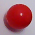
Edge Detection
I use the following Sobel operator for edge detection.
     Sy             Sx
  -1 -2 -1       -1  0  1
   0  0  0       -2  0  2
   1  2  1       -1  0  1
This gives me gradients in the same direction as the image coordinate
system: an increasing brightness from left to right gives a positive
X gradient. The same applies to the Y gradient.
By combining these two gradients, we get a gradient vector for each pixel. The size of this vector tells us whether the pixel is on an edge or not. There are two ways of calculating this size:
  [DIST1]   size=  SQRT(PX2+PY2)
  [DIST2]   size=  |PX| + |PY|
DIST1 is the correct calculation. Many people use DIST2 in order to save computation time. PX and PY are the results of the Sx and Sy operators at a given pixel. These have a maximum value of 1020 and a minimum value of -1020. For each plus and minus pair in the operators, the maximum difference we can have is 255. The sum of all positive factors is 4 in each case. Multiplying these, we get 1020. Here is a plot of the difference between DIST1 and DIST2, within the applicable range:
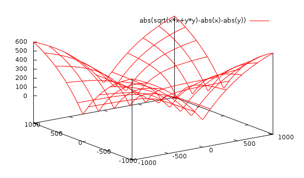
Having an accurate size for a gradient vector is quite important I think. This is because I will use some thresholding sooner or later. Accuracy of these values can make a big difference.
The maximum value of size is SQRT(2)*1020 for DIST1. This doesn't fit into 8 bits. In order to convert it to 8 bits, I can use two methods:
  [QUAN1]  size8 =  min( size , 255 )
  [QUAN2]  size8 =  size * 255 / max{∀ size}
Detecting a Circle
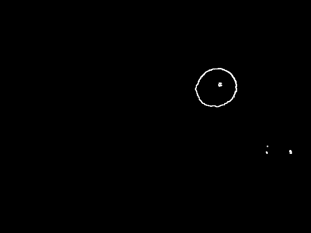
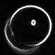
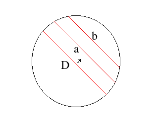
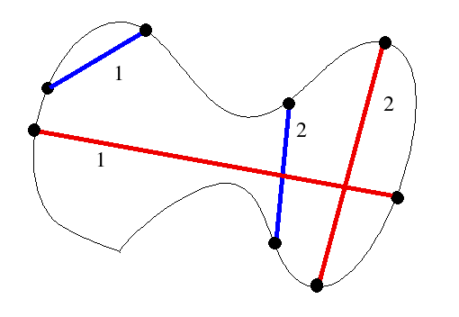
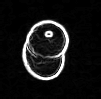
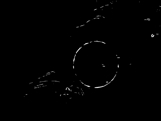
In order to detect the circle, we need to seperate it from other objects. In t10 there are three groups of connected pixels corresponding to the ball's shadow, reflection of the light source on the ball and the ball itself. I think that if there is a circle in an image, its border will always make a connected thick set of pixels. So, if I can isolate connected sets from each other I can decide whether each one corresponds to a circle or not. I will do this partition in a separate page.After I've partitioned the image into connected sets, I can find the maximally distant pair of pixels in the connected set. The line segment connecting these would be the diameter of the circle, if the set in question does correspond to a circle. By translating this diameter along its normal, I can find the intersections of the resulting line segments with the connected set. The lengths of these line segments would follow the equation for the circle if the shape is right. Here is what I mean by this:
- pick A and B
- D= distance(A,B)
- for each neighbour K of B, calculate Dk= distance(K,A)
- find K where Dk is maximum and is greater than D
- If 4 doesn't fail, set B=K and goto 2.
- If 4 fails, exchange A and B and goto 2. If this is the second failure in a row, we have found the local diameter: stop the algorithm.
Anyway, my initial thought of translating a found diameter was cute and all but not really necessary. If I have a segment which is a local diameter, then I can find its midpoint P and measure distances of the points in the set to P. If these distances are pretty much all the same, then we have a circle. Otherwise, we don't have a circle.
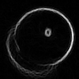
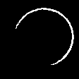
Here is the result of our example image being partitioned:


While looking for an initial pair of points, I can simply choose the top-left pixel and the bottom-right pixel. Scanning for these is very easy, I just go sequentially from the start or end of the image.
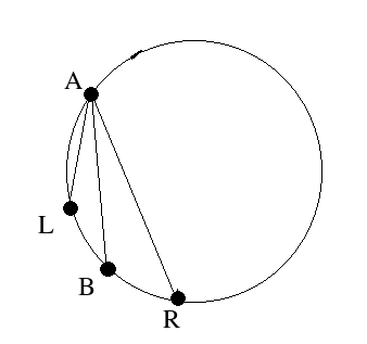
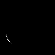
I tried my idea for finding the maximally distant pair and it failed spectacularly on t10-p1. I chose two neighbouring points in order to follow their paths, A shown in red and B shown in green.
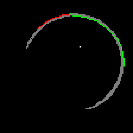
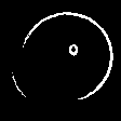
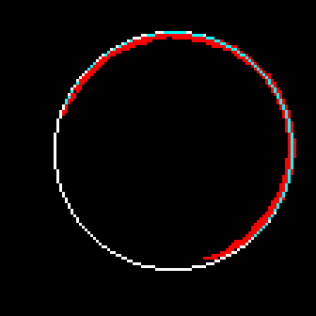
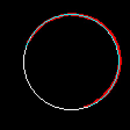
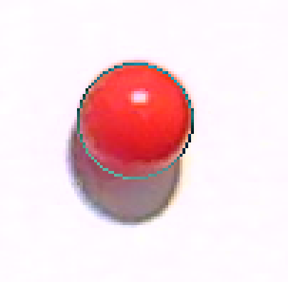
Now that I've got two points on the exterior of the circle, I can make a third one as follows. I will draw the chord AB. When I take the normal of this chord, I'm assured that it will intersect the shape since A and B are on opposite sides of the normal and they are connected. The furthest intersection is my third point. Using these three points, I can draw a circle. Below is the result, overlaid on top of t10-p1.
In order to fix this problem, I shouldn't just go with the first circle I find, but search for a better one in the neighbourhood. I will look at 27 circles total, varying the center coordinates as well as the radius by -1,0 and 1. The fitness metric will be the total luminosity value the circle accumulates over the edge pixels it passes. i.e. it will be the sum of the blue pixels in t11 over t10-p1. I have been using the result of the partitioning directly. I will now use pixels from the source image instead. Here is the REAL partitioning of t10:


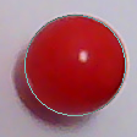
avg( abs(dist(p,center)-r) ) for p in shapeI got 1.3 for t10-x1, 1.9 for t10-x2 and 1.6 for t10-x5. I did some test with artificial images as well. I got a maximum average error of 1.73 for artificial circles. For other shapes, the average error is really high if the shape is not close to a circle. For ellipses which are really close to circles, the average error comes out as slightly above 2. So, maybe I can blindly use the value 2 for decision making.
I think I'm now ready to write the whole ball detection function. Let's review what I have done:
     X0 : input
     X1 = threshold(greyscale-red( X0 ))
     X2 = greyscale-luminosity( X0 )
     X3 = mask X2 by X1
     X4 = threshold(quant1(sobel(X3)))
     For each connected set S in X4,
       fit circle C to S
       if the average distance error in S with
          regard to C is too high, reject S
Now, I've done it. Here is a source
package for a test program. The final code is in detcir.[ch].
A New Approach
Masking the greyscale(G2) image with color information didn't work so well for scenes where there are a lot of objects near the ball I want to detect. I get a smaller image (that's not guaranteed either) but all the edges made by objects of irrelevant colors are still there and need to be eliminated. Here is an example: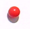
What I really need is to detect the changes in relative intensity of our target color, in this case red. Just looking at the red channel doesn't work because white also has a lot of red in it. I need to somehow suppress everything which doesn't look red. I came up with the following:
[G3] gray = RED - GREEN/2 - BLUE/2This is of course clamped to between 0 and 255. G3 is high when red component is high, unless green and blue are also high. This also suppresses dark reds to a degree. Here is the output of G3.
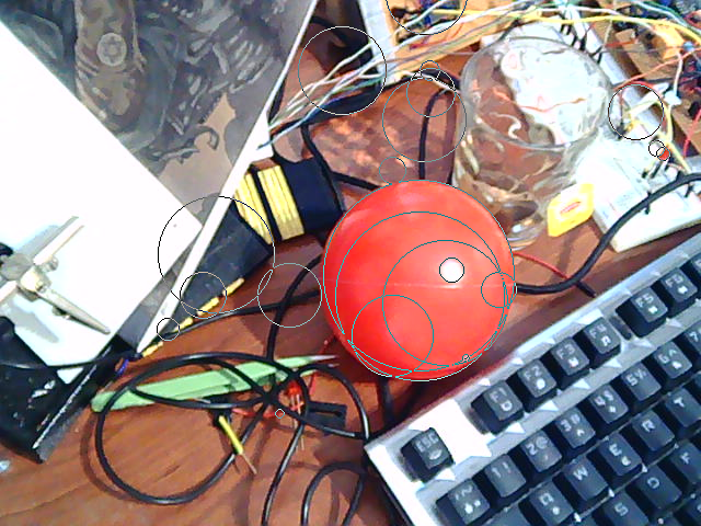
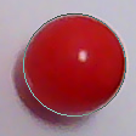
The algorithm finds a circle for almost all edges shown below. I have filtered the list of circles by hiding the ones which have a radius greater than half width of the image. These are caused by flat components.
   p0: input
   p1= G3(p0)
   p2= gauss(p1, 5, 1.0)
   p3= QUANT1(sobel(p2))
   p4= threshold(p3, 200)
   partition p4 and find circles as before
The nice thing about this is that we have only two magic numbers: color coefficient vector in G3 and the threshold value after edge detection. The former should pretty much be adjustable by examining the color of the ball to be detected. The latter is more complicated, a high value decreases the chance of detection and reduces accuracy. A low value prevents the algorithm from working at all.